Classification
The smile.classification package is a complete suite of supervised classifiers for labelling new instances with one of a discrete set of class labels. Every algorithm exposes static fit(…) factories (no mutable builders to misconfigure), accepts arbitrary integer labels, implements Classifier<T>, and is serializable.
This page walks the core abstractions (including nested Options / Properties hyperparameters), a shared 2-D visualization helper, an algorithm selection guide, then each family of methods with runnable Java / Scala / Kotlin playgrounds. Expected outputs cite unit-test metrics where available; plot demos open a Swing window.
Core Abstractions
Classifier<T> is the central contract: hard prediction (predict(x)), optional soft prediction (predict(x, posteriori)), raw score (score), and optional online update (update). Probe capabilities with isSoft() and isOnline() before calling the corresponding methods — both default to false.
// Works for any smile.classification.Classifier<T>
int label = model.predict(sample);

if (model.isSoft()) {
    double[] posteriori = new double[model.numClasses()];
    model.predict(sample, posteriori); // class probabilities
}

if (model.isOnline()) {
    model.update(newSample, newLabel); // incremental learning
}
label / optionally filled posteriori
val label = model.predict(sample)

if (model.isSoft()) {
  val posteriori = new Array[Double](model.numClasses)
  model.predict(sample, posteriori)
}

if (model.isOnline()) {
  model.update(newSample, newLabel)
}
label / optionally filled posteriori
val label = model.predict(sample)

if (model.isSoft) {
    val posteriori = DoubleArray(model.numClasses())
    model.predict(sample, posteriori)
}

if (model.isOnline) {
    model.update(newSample, newLabel)
}
label / optionally filled posteriori
DataFrameClassifier
Tree ensembles and related models implement DataFrameClassifier (extends Classifier<Tuple>). They train with a Formula plus a DataFrame, then predict named-column rows. DataFrameClassifier.of(formula, classifier) wraps any Classifier<double[]> so formula feature extraction is applied automatically.
import smile.data.formula.Formula
import smile.classification.DecisionTree

Formula formula = Formula.lhs("species");
DecisionTree tree = DecisionTree.fit(formula, data);
int[] labels = tree.predict(data);
import smile.data.formula.Formula
import smile.classification._
val formula = Formula.lhs("species")
val tree = cart(formula, data)
val labels = tree.predict(data)import smile.data.formula.Formula
import smile.classification.*
val formula = Formula.lhs("species")
val tree = cart(formula, data)
val labels = tree.predict(data)ClassLabels
Labels need not be contiguous or zero-based — {-1,+1} or {3,7,14} all work. Internally, ClassLabels remaps them to [0, k); predict always returns the original label values. ClassLabels.fit(y) also exposes priors and per-class counts.
import smile.classification.*

int[] y = {-1, +1, -1, +1};
LogisticRegression model = LogisticRegression.fit(x, y);
int label = model.predict(sample);   // returns -1 or +1

ClassLabels codec = ClassLabels.fit(y);
codec.k;       // 2
codec.priori;  // estimated class priors
import smile.classification._
val y = Array(-1, 1, -1, 1)
val model = logit(x, y)
val label = model.predict(sample) // -1 or +1
val codec = ClassLabels.fit(y)
codec.k
codec.prioriimport smile.classification.*
val y = intArrayOf(-1, 1, -1, 1)
val model = logit(x, y)
val label = model.predict(sample) // -1 or +1
val codec = ClassLabels.fit(y)
codec.k
codec.prioriOptions and Properties
Most algorithms expose a nested Options record for strongly typed hyperparameters (for example RandomForest.Options, SVM.Options, LogisticRegression.Options). Construct an Options instance and pass it to fit, or load the same knobs from a configuration file via java.util.Properties. Each Options type supports toProperties() and Options.of(props) for round-trips. Property keys use underscores (e.g. smile.random_forest.trees); algorithm sections below list the field name and the corresponding full property key in a description list.
import java.util.Properties
import smile.classification.RandomForest
import smile.data.formula.Formula

// Strongly typed Options
var options = new RandomForest.Options(200)
RandomForest model = RandomForest.fit(formula, data, options)

// Or configuration-file style Properties
Properties params = new Properties()
params.setProperty("smile.random_forest.trees", "200")
params.setProperty("smile.random_forest.max_depth", "10")
model = RandomForest.fit(formula, data, params)

// Round-trip
Properties props = options.toProperties()
var again = RandomForest.Options.of(props)
import java.util.Properties
import smile.classification._
val options = new RandomForest.Options(200)
val model = RandomForest.fit(formula, data, options)
val params = new Properties()
params.setProperty("smile.random_forest.trees", "200")
params.setProperty("smile.random_forest.max_depth", "10")
val model2 = RandomForest.fit(formula, data, params)
val props = options.toProperties
val again = RandomForest.Options.of(props)import java.util.Properties
import smile.classification.*
val options = RandomForest.Options(200)
var model = RandomForest.fit(formula, data, options)
val params = Properties()
params.setProperty("smile.random_forest.trees", "200")
params.setProperty("smile.random_forest.max_depth", "10")
model = RandomForest.fit(formula, data, params)
val props = options.toProperties()
val again = RandomForest.Options.of(props)Datasets and Visualization
Examples reuse three datasets. toy20000 is a 2-D TSV (no header; columns label, x1, x2) ideal for decision-boundary plots. For slow models, subsample the first 2000 rows for training and the next 2000 for testing — stated once here, assumed in later demos when noted. MNIST (handwritten digits) and Default (credit-card default; formula default ~ .) illustrate high-dimensional and mixed tabular Formula fits.
import smile.io.Read
import smile.datasets.*

// toy20000 — TSV, no header; columns: label, x1, x2
var toy = Read.csv("data/classification/toy20000.txt", "delimiter=\t,header=false")
double[][] x = toy.select(1, 2).toArray()
int[] y = toy.column(0).toIntArray()
// Slow models: first 2000 train / next 2000 test

var mnist = new MNIST()
double[][] mx = mnist.x()
int[] my = mnist.y()

var credit = new Default()
var formula = credit.formula()  // Formula.lhs("default")
var data = credit.data()
import smile.read
import smile.datasets._
val toy = read.csv("data/classification/toy20000.txt", delimiter = "\t", header = false)
val x = toy.select(1, 2).toArray()
val y = toy.column(0).toIntArray()
val mnist = new MNIST()
val mx = mnist.x()
val my = mnist.y()
val credit = new Default()
val formula = credit.formula // Formula.lhs("default")
val data = credit.dataimport smile.read
import smile.datasets.*
val toy = read.csv("data/classification/toy20000.txt", delimiter = "\t", header = false)
val x = toy.select(1, 2).toArray()
val y = toy.column(0).toIntArray()
val mnist = MNIST()
val mx = mnist.x()
val my = mnist.y()
val credit = Default()
val formula = credit.formula() // Formula.lhs("default")
val data = credit.data()The shared visualize helper paints a dense prediction grid, overlays a subsample of training points, and (for binary models) draws the 0.5 contour. 2-D demos below call this helper after fitting.
import smile.classification.Classifier;
import smile.math.MathEx;
import smile.plot.swing.*;

Figure visualize(Classifier<double[]> model, double[][] x, int[] y) {
    double[] lower = MathEx.colMin(x);
    double[] upper = MathEx.colMax(x);
    double[] step = { (upper[0]-lower[0])/50, (upper[1]-lower[1])/50 };
    lower[0] -= 4*step[0]; lower[1] -= 4*step[1];
    upper[0] += 4*step[0]; upper[1] += 4*step[1];

    int nx = (int) Math.round((upper[0]-lower[0])/step[0]) + 1;
    int ny = (int) Math.round((upper[1]-lower[1])/step[1]) + 1;
    double[] gx = new double[nx];
    double[] gy = new double[ny];
    for (int i = 0; i < nx; i++) gx[i] = lower[0] + i * step[0];
    for (int j = 0; j < ny; j++) gy[j] = lower[1] + j * step[1];

    double[][] grid = new double[nx*ny][2];
    for (int i = 0, k = 0; i < nx; i++)
        for (int j = 0; j < ny; j++, k++) {
            grid[k][0] = gx[i];
            grid[k][1] = gy[j];
        }
    int[] pred = model.predict(grid);
    double[][] z = new double[ny][nx];
    for (int i = 0, k = 0; i < nx; i++)
        for (int j = 0; j < ny; j++, k++)
            z[j][i] = pred[k];

    // Subsample training points for overlay clarity
    int n = Math.min(x.length, 2000);
    double[][] xs = java.util.Arrays.copyOf(x, n);
    int[] ys = java.util.Arrays.copyOf(y, n);

    var figure = ScatterPlot.of(grid, pred, '.').figure();
    figure.add(ScatterPlot.of(xs, ys, 'o'));
    if (model.numClasses() == 2)
        figure.add(new Contour(gx, gy, z, new double[]{0.5}));
    return figure;
}
Figure (call .show() to open)
import smile.classification.Classifier
import smile.math.MathEx
import smile.plot.swing._

def visualize(model: Classifier[Array[Double]], x: Array[Array[Double]], y: Array[Int]): Figure = {
  val lower = MathEx.colMin(x)
  val upper = MathEx.colMax(x)
  val step = Array((upper(0) - lower(0)) / 50, (upper(1) - lower(1)) / 50)
  lower(0) -= 4 * step(0); lower(1) -= 4 * step(1)
  upper(0) += 4 * step(0); upper(1) += 4 * step(1)

  val nx = Math.round((upper(0) - lower(0)) / step(0)).toInt + 1
  val ny = Math.round((upper(1) - lower(1)) / step(1)).toInt + 1
  val gx = Array.tabulate(nx)(i => lower(0) + i * step(0))
  val gy = Array.tabulate(ny)(j => lower(1) + j * step(1))

  val grid = Array.tabulate(nx * ny) { k =>
    val i = k / ny; val j = k % ny
    Array(gx(i), gy(j))
  }
  val pred = model.predict(grid)
  val z = Array.ofDim[Double](ny, nx)
  var k = 0
  for (i <- 0 until nx; j <- 0 until ny) {
    z(j)(i) = pred(k); k += 1
  }

  val n = math.min(x.length, 2000)
  val xs = x.take(n)
  val ys = y.take(n)

  val figure = ScatterPlot.of(grid, pred, '.').figure()
  figure.add(ScatterPlot.of(xs, ys, 'o'))
  if (model.numClasses == 2)
    figure.add(new Contour(gx, gy, z, Array(0.5)))
  figure
}
Figure (call .show() to open)
import smile.classification.Classifier
import smile.math.MathEx
import smile.plot.swing.*

fun visualize(model: Classifier<DoubleArray>, x: Array<DoubleArray>, y: IntArray): Figure {
    val lower = MathEx.colMin(x)
    val upper = MathEx.colMax(x)
    val step = doubleArrayOf((upper[0] - lower[0]) / 50, (upper[1] - lower[1]) / 50)
    lower[0] -= 4 * step[0]; lower[1] -= 4 * step[1]
    upper[0] += 4 * step[0]; upper[1] += 4 * step[1]

    val nx = Math.round((upper[0] - lower[0]) / step[0]).toInt() + 1
    val ny = Math.round((upper[1] - lower[1]) / step[1]).toInt() + 1
    val gx = DoubleArray(nx) { i -> lower[0] + i * step[0] }
    val gy = DoubleArray(ny) { j -> lower[1] + j * step[1] }

    val grid = Array(nx * ny) { k ->
        val i = k / ny; val j = k % ny
        doubleArrayOf(gx[i], gy[j])
    }
    val pred = model.predict(grid)
    val z = Array(ny) { DoubleArray(nx) }
    var k = 0
    for (i in 0 until nx) for (j in 0 until ny) {
        z[j][i] = pred[k].toDouble(); k++
    }

    val n = minOf(x.size, 2000)
    val xs = x.copyOf(n)
    val ys = y.copyOf(n)

    val figure = ScatterPlot.of(grid, pred, '.').figure()
    figure.add(ScatterPlot.of(xs, ys, 'o'))
    if (model.numClasses() == 2)
        figure.add(Contour(gx, gy, z, doubleArrayOf(0.5)))
    return figure
}
Figure (call .show() to open)
Algorithm Selection Guide
There is no universally best classifier. Use this table as a starting point.
| Situation | Recommended | Notes |
|---|---|---|
| Strong default baseline | RandomForest | Robust mixed tabular features; free OOB error. |
| Highest tuned tabular accuracy | GradientTreeBoost | Usually strongest after tuning shrinkage / trees. |
| Fast, interpretable | DecisionTree, LogisticRegression | Explainability and quick diagnostics. |
| High-dim sparse text | DiscreteNaiveBayes, SparseLogisticRegression, Maxent | Count / sparse feature spaces. |
p > n | FLD, SparseLogisticRegression | Avoid plain LDA/QDA (singular covariance). |
| Gaussian, similar covariances | LDA | Fast linear soft classifier. |
| Different class spreads | QDA / RDA | RDA blends LDA↔QDA via alpha. |
Nonlinear, moderate n | SVM (Gaussian), RBFNetwork, MLP | Scale features first. |
| Streaming / online | DiscreteNaiveBayes, LogisticRegression, MLP | Check isOnline(). |
K-Nearest Neighbors
k-NN classifies by majority vote among the k nearest training points (lazy / instance-based learning). SMILE picks a KD-tree for low-dimensional dense Euclidean data, a cover tree for higher-dimensional metric spaces, or linear search for arbitrary distances. Soft posteriors are the fraction of neighbors per class. Normalize features before use — distance methods are scale-sensitive.
On Iris, LOOCV accuracy is about 0.96 for 1-NN and 3-NN, and 0.9667 for 5-NN / 7-NN (unit tests). Larger k smooths the boundary but can blur class edges; odd k helps avoid ties in binary problems.
import smile.classification.KNN
import smile.datasets.Iris
import smile.validation.LOOCV

var iris = new Iris()
LOOCV.classification(iris.x(), iris.y(), (x, y) -> KNN.fit(x, y, 3))
accuracy ≈ 0.9600 (Iris LOOCV, 3-NN)
import smile.classification._
import smile.datasets.Iris
import smile.validation.LOOCV

val iris = new Iris()
LOOCV.classification(iris.x, iris.y, (x, y) => knn(x, y, 3))
accuracy ≈ 0.9600 (Iris LOOCV, 3-NN)
import smile.classification.*
import smile.datasets.Iris
import smile.validation.LOOCV

val iris = Iris()
LOOCV.classification(iris.x(), iris.y()) { x, y -> knn(x, y, 3) }
accuracy ≈ 0.9600 (Iris LOOCV, 3-NN)
On a MNIST subset (2500 samples in the bundled dataset), train/test split accuracy for 1-NN is typically in the mid–high 90%s — a strong non-parametric baseline before you reach for linear or tree models.
import java.util.Arrays
import smile.classification.KNN
import smile.datasets.MNIST
import smile.validation.metric.Accuracy

var mnist = new MNIST()
double[][] x = mnist.x()
int[] y = mnist.y()
int n = 2000
double[][] trainx = Arrays.copyOfRange(x, 0, n)
int[] trainy = Arrays.copyOfRange(y, 0, n)
double[][] testx = Arrays.copyOfRange(x, n, Math.min(n + 500, x.length))
int[] testy = Arrays.copyOfRange(y, n, Math.min(n + 500, y.length))
var model = KNN.fit(trainx, trainy, 1)
Accuracy.of(testy, model.predict(testx))
accuracy typically ~0.94–0.97 on this subset (varies with split)
import smile.classification._
import smile.datasets.MNIST
import smile.validation.metric.Accuracy

val mnist = new MNIST()
val x = mnist.x; val y = mnist.y
val n = 2000
val model = knn(x.take(n), y.take(n), 1)
Accuracy.of(y.slice(n, n + 500), model.predict(x.slice(n, n + 500)))
accuracy typically ~0.94–0.97 on this subset (varies with split)
import smile.classification.*
import smile.datasets.MNIST
import smile.validation.metric.Accuracy

val mnist = MNIST()
val x = mnist.x(); val y = mnist.y()
val n = 2000
val model = knn(x.copyOf(n), y.copyOf(n), 1)
Accuracy.of(y.copyOfRange(n, n + 500), model.predict(x.copyOfRange(n, n + 500)))
accuracy typically ~0.94–0.97 on this subset (varies with split)
Custom distances and prebuilt neighbor indexes are supported. You can also pass a KNNSearch (KD-tree, cover tree, LSH) when you already maintain one.
import smile.classification.KNN
import smile.math.distance.EuclideanDistance

KNN<double[]> model = KNN.fit(x, y, 5, new EuclideanDistance());
// or: new KNN<>(knnSearch, y, k)
import smile.classification._
import smile.math.distance.EuclideanDistance
val model = knn(x, y, 5, new EuclideanDistance())import smile.classification.*
import smile.math.distance.EuclideanDistance
val model = knn(x, y, 5, EuclideanDistance())import smile.io.Read
var toy = Read.csv("data/classification/toy20000.txt", "delimiter=\t,header=false")
double[][] x = toy.select(1, 2).toArray()
int[] y = toy.column(0).toIntArray()
// For slow models, use first 2000 train / next 2000 test:
// double[][] trainx = java.util.Arrays.copyOfRange(x, 0, 2000);
// int[] trainy = java.util.Arrays.copyOfRange(y, 0, 2000);
var model = KNN.fit(x, y, 3)
visualize(model, x, y).show()
(opens plot: decision boundary)
import smile.read
val toy = read.csv("data/classification/toy20000.txt", delimiter = "\t", header = false)
val x = toy.select(1, 2).toArray()
val y = toy.column(0).toIntArray()
val model = knn(x, y, 3)
visualize(model, x, y).show()
(opens plot: decision boundary)
import smile.read
val toy = read.csv("data/classification/toy20000.txt", delimiter = "\t", header = false)
val x = toy.select(1, 2).toArray()
val y = toy.column(0).toIntArray()
val model = knn(x, y, 3)
visualize(model, x, y).show()
(opens plot: decision boundary)
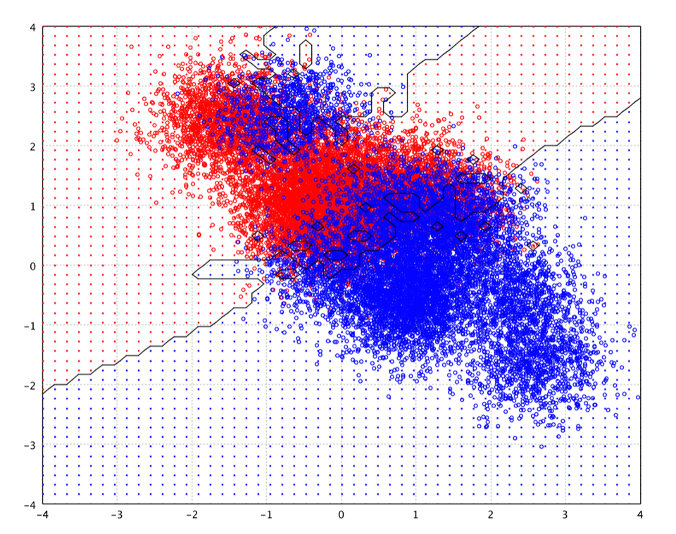
k for smoother regions.Linear Discriminant Analysis
LDA assumes class-conditional Gaussians that share a pooled covariance (homoscedastic). The decision boundary is linear. It is fast and soft (isSoft() == true). Features with variance below tol (default 1e-4) are dropped. LDA fails when p > n (singular pooled covariance) — use FLD or RDA instead.
Iris LOOCV accuracy in the unit tests is 0.8533 — lower than k-NN on this set because the Gaussian / shared-covariance assumptions are imperfect for Iris. On many near-Gaussian problems LDA remains an excellent linear baseline.
import smile.classification.LDA
import smile.datasets.Iris
import smile.validation.LOOCV

var iris = new Iris()
LOOCV.classification(iris.x(), iris.y(), (x, y) -> LDA.fit(x, y))
accuracy ≈ 0.8533 (Iris LOOCV)
import smile.classification._
import smile.datasets.Iris
import smile.validation.LOOCV

val iris = new Iris()
LOOCV.classification(iris.x, iris.y, (x, y) => lda(x, y))
accuracy ≈ 0.8533 (Iris LOOCV)
import smile.classification.*
import smile.datasets.Iris
import smile.validation.LOOCV

val iris = Iris()
LOOCV.classification(iris.x(), iris.y()) { x, y -> lda(x, y) }
accuracy ≈ 0.8533 (Iris LOOCV)
import smile.io.Read
var toy = Read.csv("data/classification/toy20000.txt", "delimiter=\t,header=false")
double[][] x = toy.select(1, 2).toArray()
int[] y = toy.column(0).toIntArray()
// For slow models, use first 2000 train / next 2000 test:
// double[][] trainx = java.util.Arrays.copyOfRange(x, 0, 2000);
// int[] trainy = java.util.Arrays.copyOfRange(y, 0, 2000);
var model = LDA.fit(x, y)
visualize(model, x, y).show()
(opens plot: decision boundary)
import smile.read
val toy = read.csv("data/classification/toy20000.txt", delimiter = "\t", header = false)
val x = toy.select(1, 2).toArray()
val y = toy.column(0).toIntArray()
val model = lda(x, y)
visualize(model, x, y).show()
(opens plot: decision boundary)
import smile.read
val toy = read.csv("data/classification/toy20000.txt", delimiter = "\t", header = false)
val x = toy.select(1, 2).toArray()
val y = toy.column(0).toIntArray()
val model = lda(x, y)
visualize(model, x, y).show()
(opens plot: decision boundary)
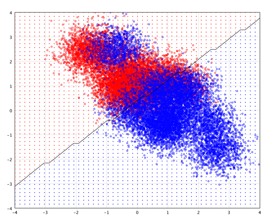
Fisher's Linear Discriminant
FLD finds a projection that maximizes between-class scatter relative to within-class scatter, then classifies by nearest projected class mean. Unlike LDA it does not require equal covariances or Gaussian classes. When n < p it uses SVD, making it the go-to linear method for the small-sample regime. Parameter L (default k − 1) is the number of discriminant directions; at most min(p, k−1) are meaningful. Soft prediction is not supported.
Iris LOOCV accuracy is about 0.98 in the unit tests.
import smile.classification.FLD
import smile.datasets.Iris
import smile.validation.LOOCV

var iris = new Iris()
LOOCV.classification(iris.x(), iris.y(), (x, y) -> FLD.fit(x, y))
// FLD.fit(x, y, L, tol);  model.project(sample)
accuracy ≈ 0.9800 (Iris LOOCV)
import smile.classification._
import smile.datasets.Iris
import smile.validation.LOOCV

val iris = new Iris()
LOOCV.classification(iris.x, iris.y, (x, y) => fisher(x, y))
accuracy ≈ 0.9800 (Iris LOOCV)
import smile.classification.*
import smile.datasets.Iris
import smile.validation.LOOCV

val iris = Iris()
LOOCV.classification(iris.x(), iris.y()) { x, y -> fisher(x, y) }
accuracy ≈ 0.9800 (Iris LOOCV)
import smile.io.Read
var toy = Read.csv("data/classification/toy20000.txt", "delimiter=\t,header=false")
double[][] x = toy.select(1, 2).toArray()
int[] y = toy.column(0).toIntArray()
// For slow models, use first 2000 train / next 2000 test:
// double[][] trainx = java.util.Arrays.copyOfRange(x, 0, 2000);
// int[] trainy = java.util.Arrays.copyOfRange(y, 0, 2000);
var model = FLD.fit(x, y)
visualize(model, x, y).show()
(opens plot: decision boundary)
import smile.read
val toy = read.csv("data/classification/toy20000.txt", delimiter = "\t", header = false)
val x = toy.select(1, 2).toArray()
val y = toy.column(0).toIntArray()
val model = fisher(x, y)
visualize(model, x, y).show()
(opens plot: decision boundary)
import smile.read
val toy = read.csv("data/classification/toy20000.txt", delimiter = "\t", header = false)
val x = toy.select(1, 2).toArray()
val y = toy.column(0).toIntArray()
val model = fisher(x, y)
visualize(model, x, y).show()
(opens plot: decision boundary)
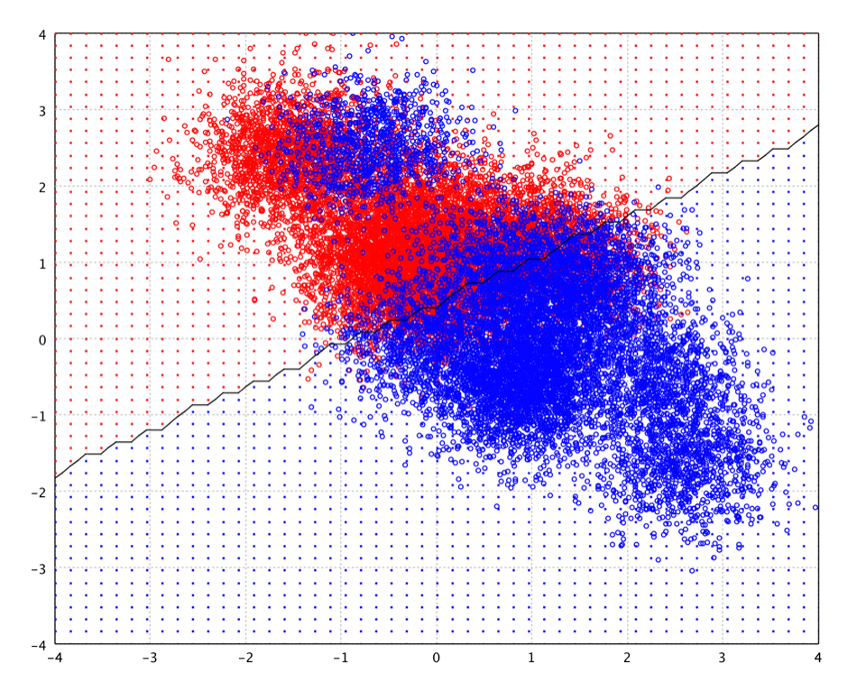
Quadratic Discriminant Analysis
QDA allows each class its own covariance, so the decision surface is quadratic. Each class needs at least p + 1 samples. It is more flexible than LDA but needs more data and is sensitive to the per-class Gaussian assumption.
import smile.io.Read
var toy = Read.csv("data/classification/toy20000.txt", "delimiter=\t,header=false")
double[][] x = toy.select(1, 2).toArray()
int[] y = toy.column(0).toIntArray()
// For slow models, use first 2000 train / next 2000 test:
// double[][] trainx = java.util.Arrays.copyOfRange(x, 0, 2000);
// int[] trainy = java.util.Arrays.copyOfRange(y, 0, 2000);
var model = QDA.fit(x, y)
visualize(model, x, y).show()
(opens plot: decision boundary)
import smile.read
val toy = read.csv("data/classification/toy20000.txt", delimiter = "\t", header = false)
val x = toy.select(1, 2).toArray()
val y = toy.column(0).toIntArray()
val model = qda(x, y)
visualize(model, x, y).show()
(opens plot: decision boundary)
import smile.read
val toy = read.csv("data/classification/toy20000.txt", delimiter = "\t", header = false)
val x = toy.select(1, 2).toArray()
val y = toy.column(0).toIntArray()
val model = qda(x, y)
visualize(model, x, y).show()
(opens plot: decision boundary)
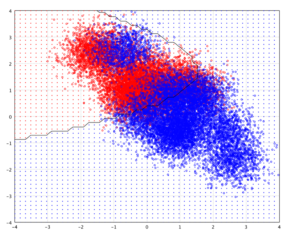
Regularized Discriminant Analysis
RDA blends LDA and QDA: Σk(α) = α Σk + (1−α) Σ. alpha = 0 recovers LDA; alpha = 1 recovers QDA. Use it when LDA's shared covariance is too strong but QDA's per-class estimates are unstable.
import smile.io.Read
var toy = Read.csv("data/classification/toy20000.txt", "delimiter=\t,header=false")
double[][] x = toy.select(1, 2).toArray()
int[] y = toy.column(0).toIntArray()
// For slow models, use first 2000 train / next 2000 test:
// double[][] trainx = java.util.Arrays.copyOfRange(x, 0, 2000);
// int[] trainy = java.util.Arrays.copyOfRange(y, 0, 2000);
var model = RDA.fit(x, y, 0.5)
visualize(model, x, y).show()
(opens plot: decision boundary)
import smile.read
val toy = read.csv("data/classification/toy20000.txt", delimiter = "\t", header = false)
val x = toy.select(1, 2).toArray()
val y = toy.column(0).toIntArray()
val model = rda(x, y, 0.5)
visualize(model, x, y).show()
(opens plot: decision boundary)
import smile.read
val toy = read.csv("data/classification/toy20000.txt", delimiter = "\t", header = false)
val x = toy.select(1, 2).toArray()
val y = toy.column(0).toIntArray()
val model = rda(x, y, 0.5)
visualize(model, x, y).show()
(opens plot: decision boundary)
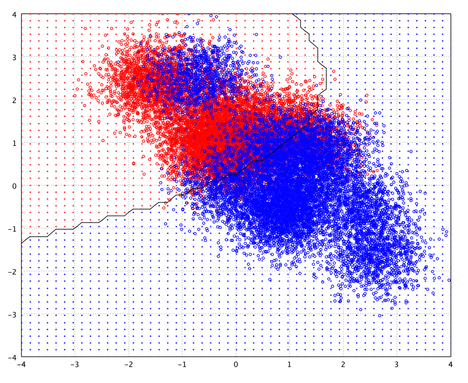
alpha = 0.5 on the toy set — between LDA and QDA.Naive Bayes
General Naive Bayes accepts arbitrary Distribution objects for each (class, feature) pair — any distribution from smile.stat.distribution. Soft prediction uses a log-sum-exp trick; online update is not supported. On Iris with 3-component Gaussian mixtures per feature, LOOCV accuracy is about 0.9533.
import java.util.stream.IntStream
import smile.classification.NaiveBayes
import smile.datasets.Iris
import smile.math.MathEx
import smile.stat.distribution.*

var iris = new Iris()
double[][] data = iris.x()
int[] label = iris.y()
int p = data[0].length, k = MathEx.max(label) + 1

double[] priori = new double[k]
Distribution[][] condprob = new Distribution[k][p]
for (int i = 0; i < k; i++) {
    priori[i] = 1.0 / k
    final int c = i
    for (int j = 0; j < p; j++) {
        final int f = j
        double[] xi = IntStream.range(0, data.length)
            .filter(l -> label[l] == c).mapToDouble(l -> data[l][f]).toArray()
        condprob[i][j] = GaussianMixture.fit(3, xi)
    }
}
var model = new NaiveBayes(priori, condprob)
model.predict(data[0])
Iris LOOCV with this setup ≈ 0.9533
import smile.classification._
import smile.datasets.Iris
import smile.math.MathEx
import smile.stat.distribution._

val iris = new Iris()
val data = iris.x
val label = iris.y
val p = data(0).length
val k = MathEx.max(label) + 1

val priori = Array.fill(k)(1.0 / k)
val condprob = Array.tabulate(k, p) { (i, j) =>
  val xi = data.zip(label).collect { case (x, y) if y == i => x(j) }
  GaussianMixture.fit(3, xi)
}
val model = naiveBayes(priori, condprob)
model.predict(data(0))
Iris LOOCV with this setup ≈ 0.9533
import smile.classification.*
import smile.datasets.Iris
import smile.math.MathEx
import smile.stat.distribution.*

val iris = Iris()
val data = iris.x()
val label = iris.y()
val p = data[0].size
val k = MathEx.max(label) + 1

val priori = DoubleArray(k) { 1.0 / k }
val condprob = Array(k) { c ->
    Array(p) { f ->
        val xi = data.indices.filter { label[it] == c }
            .map { data[it][f] }.toDoubleArray()
        GaussianMixture.fit(3, xi)
    }
}
val model = naiveBayes(priori, condprob)
model.predict(data[0])
Iris LOOCV with this setup ≈ 0.9533
Discrete Naive Bayes
Optimized for document classification on term-count vectors (int[] or SparseArray). Six generative models: MULTINOMIAL, BERNOULLI, POLYAURN, CNB, WCNB, and TWCNB (batch-only). Add-sigma smoothing defaults to 1 (Laplace). Most variants support online update; TWCNB does not. There is no nested Options record — parameters are constructor arguments:
import smile.classification.DiscreteNaiveBayes
import smile.classification.DiscreteNaiveBayes.Model

// k classes, p vocabulary size
var nb = new DiscreteNaiveBayes(Model.MULTINOMIAL, k, p)
nb.update(x, y)          // int[][] x, int[] y  (or SparseArray)
int label = nb.predict(doc)
double[] post = new double[k]
nb.predict(doc, post)    // soft prediction

// TWCNB generally best on text but batch-only
var tw = new DiscreteNaiveBayes(Model.TWCNB, k, p)
import smile.classification._
import smile.classification.DiscreteNaiveBayes.Model
val nb = naiveBayes(x, y, Model.MULTINOMIAL) // trains via update
val label = nb.predict(doc)import smile.classification.*
import smile.classification.DiscreteNaiveBayes.Model
val nb = naiveBayes(x, y, Model.MULTINOMIAL) // trains via update
val label = nb.predict(doc)Maximum Entropy
Maxent is multinomial logistic regression over sparse integer-indexed binary features (classic NLP feature templates). Pass feature-space size p and int[][] (or SparseArray[]) samples. Optimized by L-BFGS; also supports online SGD updates.
Hyperparameters are fields of the nested Maxent.Options record. Pass an Options instance to fit, or a java.util.Properties map using the keys below (Options.toProperties() / Options.of(props) round-trip).
import smile.classification.Maxent

var options = new Maxent.Options(0.1, 1E-5, 500)
Maxent model = Maxent.fit(p, x, y, options)  // x: int[][]
double[] post = new double[model.numClasses()]
int label = model.predict(sample, post)
import smile.classification._
val model = maxent(x, y, p, lambda = 0.1)
val label = model.predict(sample)import smile.classification.*
val model = maxent(x, y, p, lambda = 0.1)
val label = model.predict(sample)Logistic Regression
Penalized maximum-likelihood logistic regression via L-BFGS. Binary problems use the Binomial subclass; multiclass uses Multinomial. Soft prediction, AIC/BIC, and online SGD updates are supported. Iris LOOCV accuracy is about 0.9667.
Hyperparameters are fields of the nested LogisticRegression.Options record. Pass an Options instance to fit, or a java.util.Properties map using the keys below (Options.toProperties() / Options.of(props) round-trip).
import smile.classification.LogisticRegression
import smile.datasets.Iris
import smile.validation.LOOCV

var iris = new Iris()
var options = new LogisticRegression.Options(0.1, 1E-5, 500)
LOOCV.classification(iris.x(), iris.y(),
    (x, y) -> LogisticRegression.fit(x, y, options))
accuracy ≈ 0.9667 (Iris LOOCV)
import smile.classification._
import smile.datasets.Iris
import smile.validation.LOOCV

val iris = new Iris()
LOOCV.classification(iris.x, iris.y, (x, y) => logit(x, y, lambda = 0.1))
accuracy ≈ 0.9667 (Iris LOOCV)
import smile.classification.*
import smile.datasets.Iris
import smile.validation.LOOCV

val iris = Iris()
LOOCV.classification(iris.x(), iris.y()) { x, y -> logit(x, y, lambda = 0.1) }
accuracy ≈ 0.9667 (Iris LOOCV)
import smile.io.Read
var toy = Read.csv("data/classification/toy20000.txt", "delimiter=\t,header=false")
double[][] x = toy.select(1, 2).toArray()
int[] y = toy.column(0).toIntArray()
// For slow models, use first 2000 train / next 2000 test:
// double[][] trainx = java.util.Arrays.copyOfRange(x, 0, 2000);
// int[] trainy = java.util.Arrays.copyOfRange(y, 0, 2000);
var model = LogisticRegression.fit(x, y)
visualize(model, x, y).show()
(opens plot: decision boundary)
import smile.read
val toy = read.csv("data/classification/toy20000.txt", delimiter = "\t", header = false)
val x = toy.select(1, 2).toArray()
val y = toy.column(0).toIntArray()
val model = logit(x, y)
visualize(model, x, y).show()
(opens plot: decision boundary)
import smile.read
val toy = read.csv("data/classification/toy20000.txt", delimiter = "\t", header = false)
val x = toy.select(1, 2).toArray()
val y = toy.column(0).toIntArray()
val model = logit(x, y)
visualize(model, x, y).show()
(opens plot: decision boundary)
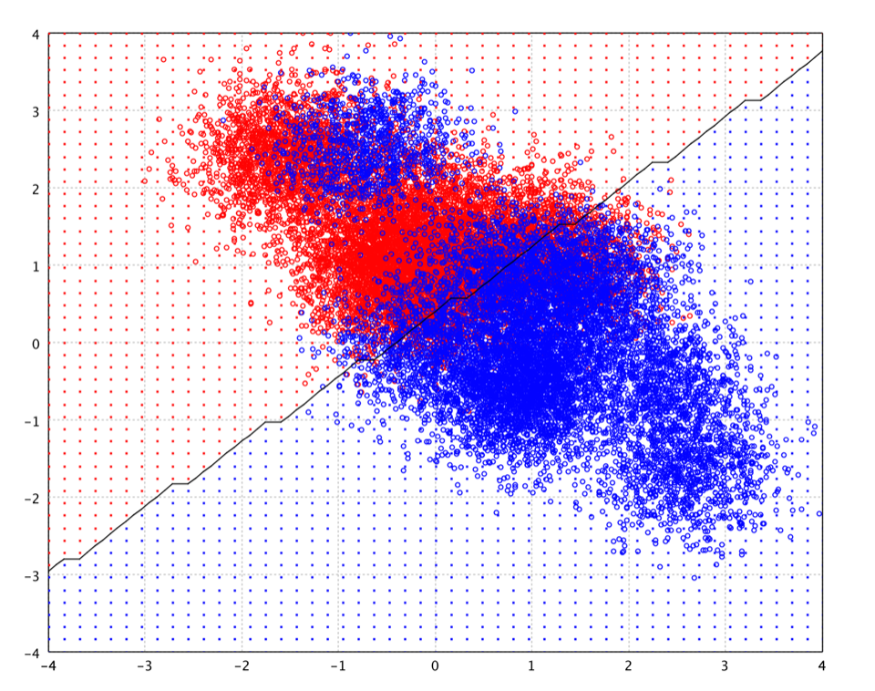
Sparse Logistic Regression
Same objective as logistic regression, but trained on SparseDataset<Integer> — suitable for high-dimensional bag-of-words. Reuse LogisticRegression.Options (and the same smile.logistic.* property keys) for hyperparameters. Online update(SparseArray, int) is supported.
import java.util.stream.IntStream
import smile.classification.*
import smile.data.*
import smile.util.SparseArray

SparseDataset<Integer> sparse = new SparseDataset<>(
    IntStream.range(0, x.length).mapToObj(i -> {
        SparseArray a = new SparseArray();
        for (int j = 0; j < x[i].length; j++)
            if (x[i][j] != 0.0) a.append(j, x[i][j]);
        return new SampleInstance<>(a, y[i]);
    }).toList()
);
var options = new LogisticRegression.Options(0.3, 1E-3, 1000);
SparseLogisticRegression model = SparseLogisticRegression.fit(sparse, options);
import smile.classification._
import smile.data._
import smile.util.SparseArray
import scala.jdk.CollectionConverters._
val instances = x.indices.map { i =>
val a = new SparseArray
x(i).indices.filter(x(i)(_) != 0.0).foreach(j => a.append(j, x(i)(j)))
new SampleInstance(a, Integer.valueOf(y(i)))
}.asJava
val sparse = new SparseDataset[Integer](instances)
val model = SparseLogisticRegression.fit(sparse,
new LogisticRegression.Options(0.3, 1E-3, 1000))import smile.classification.*
import smile.data.*
import smile.util.SparseArray
val instances = x.indices.map { i ->
val a = SparseArray()
x[i].indices.filter { x[i][it] != 0.0 }.forEach { j -> a.append(j, x[i][j]) }
SampleInstance(a, y[i])
}
val sparse = SparseDataset(java.util.ArrayList(instances))
val model = SparseLogisticRegression.fit(
sparse, LogisticRegression.Options(0.3, 1E-3, 1000))Multilayer Perceptron
A fully connected feed-forward net trained by stochastic back-propagation. Build layers with Layer.input, hidden activations (sigmoid, ReLU, tanh, …), and Layer.mle(k, OutputFunction.SOFTMAX) for multiclass, then call update for epochs — or use MLP.fit(x, y, Properties) with smile.mlp.layers like "ReLU(100)". Scale inputs to similar ranges. Soft prediction and online updates are supported.
MLP is configured primarily through java.util.Properties (or setters on the trained network). Keys used by fit(…, Properties) / setParameters:
import smile.classification.MLP
import smile.model.mlp.*
import smile.util.function.TimeFunction

int p = x[0].length, k = 3  // feature dim / classes
var net = new MLP(
    Layer.input(p),
    Layer.sigmoid(50),
    Layer.mle(k, OutputFunction.SOFTMAX)
)
net.setLearningRate(TimeFunction.constant(0.01))
for (int epoch = 0; epoch < 20; epoch++)
    net.update(x, y)

// Or: MLP.fit(x, y, props) with smile.mlp.layers=ReLU(100)
import smile.classification._
import smile.model.mlp._
val net = mlp(x, y, Array(Layer.input(p), Layer.sigmoid(50),
Layer.mle(k, OutputFunction.SOFTMAX)), epochs = 20)import smile.classification.*
import smile.model.mlp.*
val net = mlp(x, y, arrayOf(Layer.input(p), Layer.sigmoid(50),
Layer.mle(k, OutputFunction.SOFTMAX)), epochs = 20)Radial Basis Function Network
A two-layer model: RBF activations at k-means (or supplied) centers, then a linear least-squares output. Gaussian RBF networks via RBF.fit(x, k) are the usual starting point; set normalized = true for NRBF. Soft prediction and online updates are not supported. Iris LOOCV with 10 centers is about 0.9733 (normalized ≈ 0.9867).
import smile.classification.RBFNetwork
import smile.model.rbf.RBF
import smile.datasets.Iris
import smile.validation.LOOCV

var iris = new Iris()
LOOCV.classification(iris.x(), iris.y(), (x, y) -> {
    var neurons = RBF.fit(x, 10);
    return RBFNetwork.fit(x, y, neurons);
})
accuracy ≈ 0.9733 (Iris LOOCV, 10 centers)
import smile.classification._
import smile.datasets.Iris
import smile.validation.LOOCV

val iris = new Iris()
LOOCV.classification(iris.x, iris.y, (x, y) => rbfnet(x, y, 10))
accuracy ≈ 0.9733 (Iris LOOCV, 10 centers)
import smile.classification.*
import smile.datasets.Iris
import smile.validation.LOOCV

val iris = Iris()
LOOCV.classification(iris.x(), iris.y()) { x, y -> rbfnet(x, y, 10) }
accuracy ≈ 0.9733 (Iris LOOCV, 10 centers)
import smile.io.Read
var toy = Read.csv("data/classification/toy20000.txt", "delimiter=\t,header=false")
double[][] x = toy.select(1, 2).toArray()
int[] y = toy.column(0).toIntArray()
// For slow models, use first 2000 train / next 2000 test:
// double[][] trainx = java.util.Arrays.copyOfRange(x, 0, 2000);
// int[] trainy = java.util.Arrays.copyOfRange(y, 0, 2000);
var neurons = smile.model.rbf.RBF.fit(x, 20);
var model = RBFNetwork.fit(x, y, neurons)
visualize(model, x, y).show()
(opens plot: decision boundary)
import smile.read
val toy = read.csv("data/classification/toy20000.txt", delimiter = "\t", header = false)
val x = toy.select(1, 2).toArray()
val y = toy.column(0).toIntArray()
val model = rbfnet(x, y, 20)
visualize(model, x, y).show()
(opens plot: decision boundary)
import smile.read
val toy = read.csv("data/classification/toy20000.txt", delimiter = "\t", header = false)
val x = toy.select(1, 2).toArray()
val y = toy.column(0).toIntArray()
val model = rbfnet(x, y, 20)
visualize(model, x, y).show()
(opens plot: decision boundary)
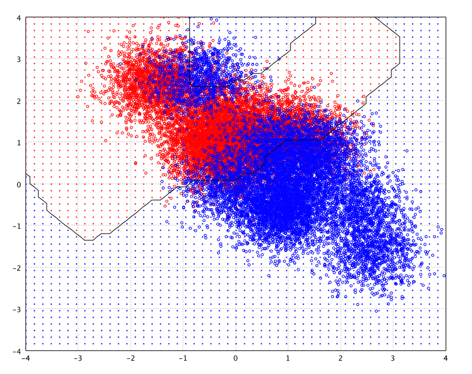
Support Vector Machines
Binary kernel SVM trained with LASVM. Labels must be +1 / −1. Choose a Mercer kernel (linear, Gaussian, polynomial, Laplacian, …) and soft-margin C. model.score(x) is the signed distance to the hyperplane. Multiclass problems use OvO / OvR (below) or SVM.fit(x, y, Properties) with smile.svm.multiclass=OVO|OVR.
Hyperparameters are fields of the nested SVM.Options record. Pass an Options instance to fit, or a java.util.Properties map using the keys below (Options.toProperties() / Options.of(props) round-trip). Linear / sparse linear SVM fits reuse the same SVM.Options and keys.
import smile.classification.SVM
import smile.math.kernel.GaussianKernel

// Remap labels to +1 / -1 if needed
var options = new SVM.Options(1.0)  // C=1, tol=1E-3, epochs=1
SVM<double[]> model = SVM.fit(x, y, new GaussianKernel(1.0), options)
double score = model.score(sample)
int label = model.predict(sample)
import smile.classification._
import smile.math.kernel.GaussianKernel
val model = svm(x, y, new GaussianKernel(1.0), C = 1.0)
val score = model.score(sample)import smile.classification.*
import smile.math.kernel.GaussianKernel
val model = svm(x, y, GaussianKernel(1.0), C = 1.0)
val score = model.score(sample)import smile.io.Read
var toy = Read.csv("data/classification/toy20000.txt", "delimiter=\t,header=false")
double[][] x = toy.select(1, 2).toArray()
int[] y = toy.column(0).toIntArray()
// For slow models, use first 2000 train / next 2000 test:
// double[][] trainx = java.util.Arrays.copyOfRange(x, 0, 2000);
// int[] trainy = java.util.Arrays.copyOfRange(y, 0, 2000);
// Ensure +1/-1 labels for binary SVM
int[] ypm = java.util.Arrays.stream(y).map(yi -> yi == 0 ? -1 : 1).toArray();
var model = SVM.fit(x, ypm, new smile.math.kernel.GaussianKernel(0.5), new SVM.Options(1.0));
visualize(model, x, y).show()
(opens plot: decision boundary)
import smile.read
val toy = read.csv("data/classification/toy20000.txt", delimiter = "\t", header = false)
val x = toy.select(1, 2).toArray()
val y = toy.column(0).toIntArray()
val ypm = y.map(yi => if (yi == 0) -1 else 1)
val model = svm(x, ypm, new smile.math.kernel.GaussianKernel(0.5), 1.0)
visualize(model, x, y).show()
(opens plot: decision boundary)
import smile.read
val toy = read.csv("data/classification/toy20000.txt", delimiter = "\t", header = false)
val x = toy.select(1, 2).toArray()
val y = toy.column(0).toIntArray()
val ypm = IntArray(y.size) { if (y[it] == 0) -1 else 1 }
val model = svm(x, ypm, smile.math.kernel.GaussianKernel(0.5), 1.0)
visualize(model, x, y).show()
(opens plot: decision boundary)
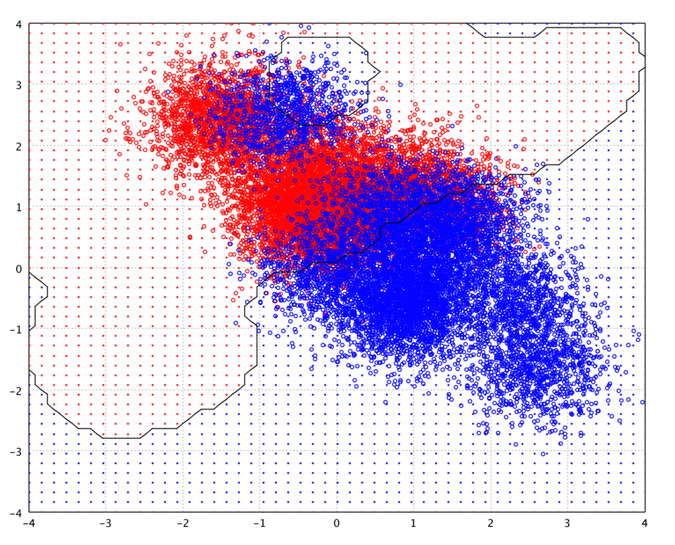
Linear SVM and Sparse Variants
SVM.fit(x, y, options) with a linear kernel returns a LinearSVM exposing weights() and intercept(). SparseLinearSVM and BinarySparseLinearSVM are the sparse and binary-sparse counterparts — useful when you need to inspect or export the linear decision boundary.
import smile.classification.SVM
import smile.classification.LinearSVM

LinearSVM model = SVM.fit(x, y, new SVM.Options(1.0)); // +1/-1 labels
double[] w = model.weights();
double b = model.intercept();
double s = model.score(sample);  // w·x + b

// SparseLinearSVM.fit(sparseX, y, p, options)
// BinarySparseLinearSVM.fit(intX, y, p, options)
import smile.classification.SVM
import smile.classification.LinearSVM
val model: LinearSVM = SVM.fit(x, y, new SVM.Options(1.0))
val w = model.weights
val b = model.interceptimport smile.classification.SVM
import smile.classification.LinearSVM
val model: LinearSVM = SVM.fit(x, y, SVM.Options(1.0))
val w = model.weights()
val b = model.intercept()One-Versus-Rest and One-Versus-One
Both strategies reduce a k-class problem to binary trainers (k ≥ 3). OvR trains k classifiers (class i vs rest) and picks the highest Platt-scaled score — the base trainer should support score() or soft prediction will be unavailable. OvO trains k(k−1)/2 pairwise classifiers; hard prediction always works via majority vote. Prefer OvO for SVMs; OvR for calibrated soft models like logistic regression.
import smile.classification.*
import smile.math.kernel.GaussianKernel

// OvR with logistic regression
OneVersusRest<double[]> ovr = OneVersusRest.fit(x, y,
    (a, b) -> LogisticRegression.fit(a, b));

// OvO with SVM (+1/-1 binary labels inside)
OneVersusOne<double[]> ovo = OneVersusOne.fit(x, y,
    (a, b) -> SVM.fit(a, b, new GaussianKernel(1.0), new SVM.Options(1.0)));

int label = ovo.predict(sample);  // voting always works
if (ovr.isSoft()) {
    double[] post = new double[ovr.numClasses()];
    ovr.predict(sample, post);
}
import smile.classification._
import smile.math.kernel.GaussianKernel
val ovr = ovr(x, y) { (a, b) => logit(a, b) }
val ovo = ovo(x, y) { (a, b) =>
svm(a, b, new GaussianKernel(1.0), 1.0)
}
val label = ovo.predict(sample)import smile.classification.*
import smile.math.kernel.GaussianKernel
val ovrModel = ovr(x, y) { a, b -> logit(a, b) }
val ovoModel = ovo(x, y) { a, b ->
svm(a, b, GaussianKernel(1.0), 1.0)
}
val label = ovoModel.predict(sample)Probability Calibration
Raw scores are not always calibrated probabilities. Platt scaling fits P = 1 / (1 + exp(A·f + B)) — the standard post-process for SVMs. Isotonic regression (PAV) fits a monotone step function and needs more data but handles non-logistic score→probability maps. Fit on a held-out calibration set; labels for Platt use positive / non-positive convention.
import smile.classification.*

LogisticRegression base = LogisticRegression.fit(xTrain, yTrain);

// From classifier scores
PlattScaling ps = PlattScaling.fit(base, xCal, yCal);
double prob = ps.scale(base.score(testSample));

// Or from raw scores / isotonic
// PlattScaling.fit(scores, labels);
IsotonicRegressionScaling irs = IsotonicRegressionScaling.fit(scores, labels);
double p2 = irs.scale(score);
import smile.classification._
val base = logit(xTrain, yTrain)
val ps = PlattScaling.fit(base, xCal, yCal)
val prob = ps.scale(base.score(testSample))
val irs = IsotonicRegressionScaling.fit(scores, labels)import smile.classification.*
val base = logit(xTrain, yTrain)
val ps = PlattScaling.fit(base, xCal, yCal)
val prob = ps.scale(base.score(testSample))
val irs = IsotonicRegressionScaling.fit(scores, labels)Decision Trees
CART trees operate on Tuple / DataFrame data through a Formula. They handle mixed numeric and categorical features without scaling, produce interpretable rules, and expose Gini importance — but overfit easily alone. Prefer ensembles in production.
Hyperparameters are fields of the nested DecisionTree.Options record. Pass an Options instance to fit, or a java.util.Properties map using the keys below (Options.toProperties() / Options.of(props) round-trip).
import smile.classification.DecisionTree
import smile.data.DataFrame
import smile.data.formula.Formula
import smile.data.vector.IntVector
import smile.model.cart.SplitRule
import smile.io.Read

var toy = Read.csv("data/classification/toy20000.txt", "delimiter=\t,header=false")
double[][] x = toy.select(1, 2).toArray()
int[] y = toy.column(0).toIntArray()
// Subsample for speed
x = java.util.Arrays.copyOf(x, 2000)
y = java.util.Arrays.copyOf(y, 2000)

DataFrame data = DataFrame.of(x, "x1", "x2").add(new IntVector("y", y))
Formula formula = Formula.lhs("y")
var options = new DecisionTree.Options(SplitRule.GINI, 10, 0, 5)
DecisionTree model = DecisionTree.fit(formula, data, options)
model.importance()
import smile.classification._
import smile.data._
import smile.data.formula.Formula
import smile.data.vector.IntVector
import smile.model.cart.SplitRule
import smile.read
val toy = read.csv("data/classification/toy20000.txt", delimiter = "\t", header = false)
val x = toy.select(1, 2).toArray().take(2000)
val y = toy.column(0).toIntArray().take(2000)
val data = DataFrame.of(x, "x1", "x2").add(new IntVector("y", y))
val formula = Formula.lhs("y")
val model = cart(formula, data, SplitRule.GINI, maxDepth = 10)
model.importanceimport smile.classification.*
import smile.data.DataFrame
import smile.data.formula.Formula
import smile.data.vector.IntVector
import smile.model.cart.SplitRule
import smile.read
val toy = read.csv("data/classification/toy20000.txt", delimiter = "\t", header = false)
val x = toy.select(1, 2).toArray().copyOf(2000)
val y = toy.column(0).toIntArray().copyOf(2000)
val data = DataFrame.of(x, "x1", "x2").add(IntVector("y", y))
val formula = Formula.lhs("y")
val model = cart(formula, data, SplitRule.GINI, maxDepth = 10)
model.importance()On the credit-default dataset, Formula fits are the natural API:
import smile.classification.DecisionTree
import smile.datasets.Default

var credit = new Default()
DecisionTree tree = DecisionTree.fit(credit.formula(), credit.data())
int[] pred = tree.predict(credit.data())
import smile.classification._
import smile.datasets.Default
val credit = new Default()
val tree = cart(credit.formula, credit.data)
val pred = tree.predict(credit.data)import smile.classification.*
import smile.datasets.Default
val credit = Default()
val tree = cart(credit.formula(), credit.data())
val pred = tree.predict(credit.data())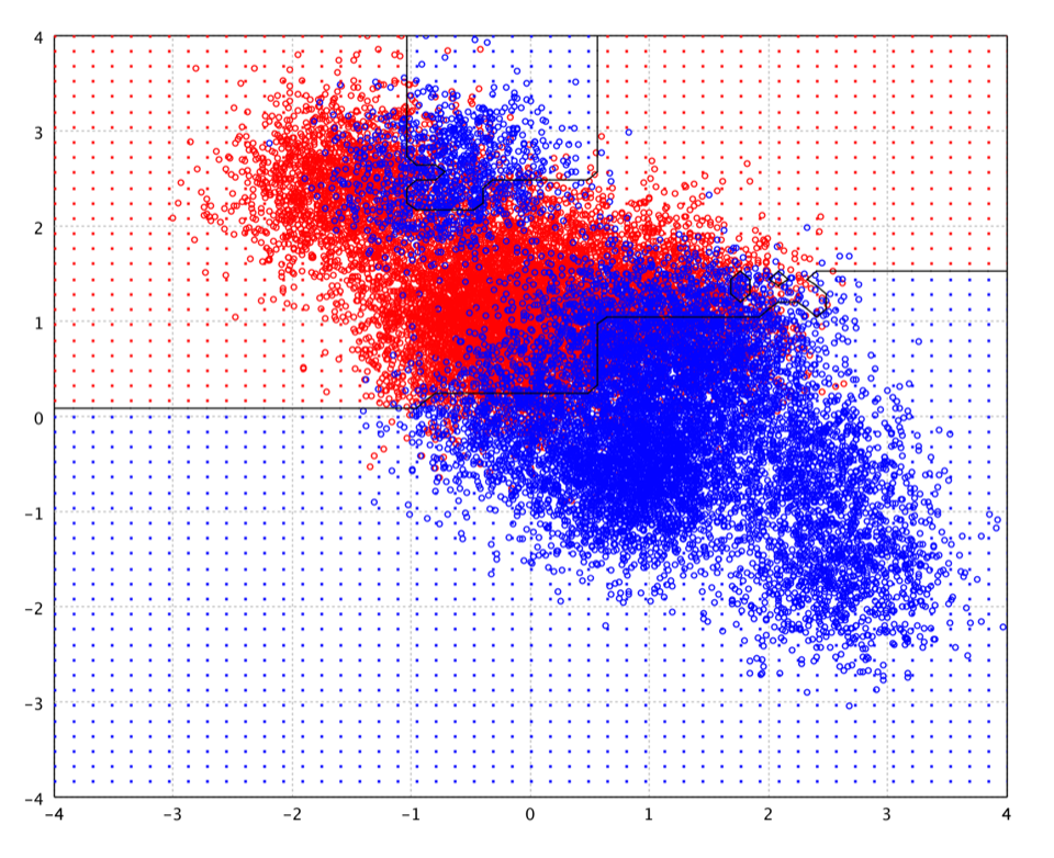
Random Forest
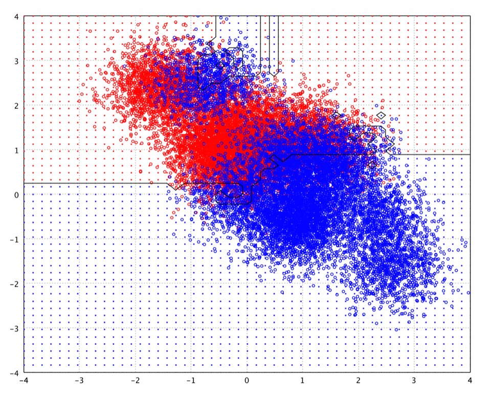
An ensemble of trees grown on bootstrap samples with random feature subsets at each split. Majority vote (optionally OOB-weighted) gives the prediction. OOB samples yield a nearly free unbiased accuracy estimate via model.metrics(). Iris LOOCV with a modest forest is about 0.9533.
Hyperparameters are fields of the nested RandomForest.Options record. Pass an Options instance to fit, or a java.util.Properties map using the keys below (Options.toProperties() / Options.of(props) round-trip).
import smile.classification.RandomForest
import smile.datasets.*
import smile.math.MathEx

MathEx.setSeed(19650218)
var iris = new Iris()
var options = new RandomForest.Options(100)
RandomForest model = RandomForest.fit(iris.formula(), iris.data(), options)
System.out.println(model.metrics())  // OOB accuracy, etc.
model.importance()

// Tabular credit default
var credit = new Default()
RandomForest rf = RandomForest.fit(credit.formula(), credit.data(),
    new RandomForest.Options(200));
Iris LOOCV ≈ 0.9533; inspect model.metrics() for OOB
import smile.classification._
import smile.datasets._
import smile.math.MathEx

MathEx.setSeed(19650218)
val iris = new Iris()
val model = randomForest(iris.formula, iris.data, ntrees = 100)
println(model.metrics)
model.importance

val credit = new Default()
val rf = randomForest(credit.formula, credit.data, ntrees = 200)
Iris LOOCV ≈ 0.9533; inspect model.metrics() for OOB
import smile.classification.*
import smile.datasets.*
import smile.math.MathEx

MathEx.setSeed(19650218)
val iris = Iris()
val model = randomForest(iris.formula(), iris.data(), ntrees = 100)
println(model.metrics())
model.importance()

val credit = Default()
val rf = randomForest(credit.formula(), credit.data(), ntrees = 200)
Iris LOOCV ≈ 0.9533; inspect model.metrics() for OOB
Gradient Tree Boost
Gradient boosting fits regression trees to pseudo-residuals. Shrinkage (learning rate) trades off against tree count: smaller shrinkage needs more trees but usually generalizes better. Stochastic subsampling (subsample < 1) adds regularization. Often the strongest tabular accuracy after tuning.
Hyperparameters are fields of the nested GradientTreeBoost.Options record. Pass an Options instance to fit, or a java.util.Properties map using the keys below (Options.toProperties() / Options.of(props) round-trip).
import smile.classification.GradientTreeBoost
import smile.datasets.Iris
import smile.math.MathEx

MathEx.setSeed(19650218)
var iris = new Iris()
var options = new GradientTreeBoost.Options(100)
GradientTreeBoost model = GradientTreeBoost.fit(
    iris.formula(), iris.data(), options)
model.importance()
import smile.classification._
import smile.datasets.Iris
import smile.math.MathEx
MathEx.setSeed(19650218)
val iris = new Iris()
val model = gbm(iris.formula, iris.data, ntrees = 100)
model.importanceimport smile.classification.*
import smile.datasets.Iris
import smile.math.MathEx
MathEx.setSeed(19650218)
val iris = Iris()
val model = gbm(iris.formula(), iris.data(), ntrees = 100)
model.importance()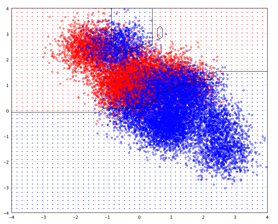
AdaBoost
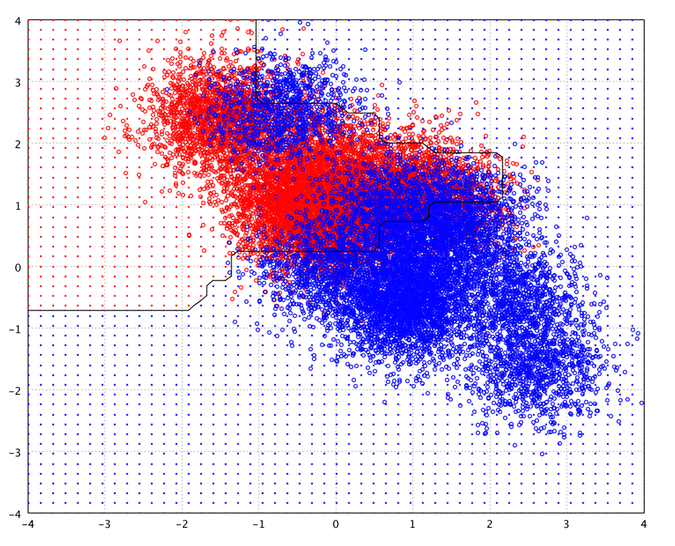
Adaptive boosting iteratively reweights misclassified samples (SAMME for multiclass). Sensitive to label noise and outliers because hard examples keep gaining weight, but often less overfit-prone than a single deep tree. Iris LOOCV accuracy is about 0.9533.
Hyperparameters are fields of the nested AdaBoost.Options record. Pass an Options instance to fit, or a java.util.Properties map using the keys below (Options.toProperties() / Options.of(props) round-trip).
import smile.classification.AdaBoost
import smile.datasets.Iris
import smile.math.MathEx

MathEx.setSeed(19650218)
var iris = new Iris()
AdaBoost model = AdaBoost.fit(iris.formula(), iris.data(),
    new AdaBoost.Options(100))
model.importance()
Iris LOOCV ≈ 0.9533
import smile.classification._
import smile.datasets.Iris
import smile.math.MathEx

MathEx.setSeed(19650218)
val iris = new Iris()
val model = adaboost(iris.formula, iris.data, ntrees = 100)
model.importance
Iris LOOCV ≈ 0.9533
import smile.classification.*
import smile.datasets.Iris
import smile.math.MathEx

MathEx.setSeed(19650218)
val iris = Iris()
val model = adaboost(iris.formula(), iris.data(), ntrees = 100)
model.importance()
Iris LOOCV ≈ 0.9533
Practical Tips
- Probe capabilities. Call
isSoft()/isOnline()before soft predict or update. - Arbitrary labels. Any integers work;
predictreturns original values. - Validation. Prefer
CrossValidation.classificationorLOOCV.classification(andAccuracy) over hand-rolled holdouts; seed withMathEx.setSeed(…)for reproducible ensembles and folds. - Formula vs arrays. Use
Formula+DataFramefor mixed/categorical tabular data (trees, ensembles); usedouble[][]for numeric feature matrices and distance / kernel methods. - Class imbalance. See
smile.classification.resampling(SMOTE, ADASYN, Tomek links, …) before tuning the classifier. - Scale-sensitive models. Normalize for LDA/QDA/RDA/FLD, logistic, k-NN, SVM, MLP, RBF. Trees and DiscreteNaiveBayes are scale-invariant.
- Serialize.
Write.object(model, path)/Read.object(path). - Properties configs. Prefer nested
Optionswhen coding; use the property keys listed under each algorithm (underscores, e.g.smile.random_forest.trees) for configuration files. Round-trip withtoProperties()/Options.of(props). - Large
n. Prefer tree ensembles; kernel SVM scales poorly. Forp > n, prefer FLD / sparse logistic / Maxent. - Calibration. Platt or isotonic on a held-out set when you need trustworthy probabilities from score-based models.