Manifold Learning

Overview

Manifold learning finds a low-dimensional basis for describing high-dimensional data. Though each point may have thousands of features, the data often lie on (or near) a low-dimensional manifold embedded in that high-dimensional space. Manifold algorithms recover coordinates on that manifold for visualization and downstream analysis.

SMILE’s nonlinear embedding methods live in smile.manifold: IsoMap, LLE, Laplacian Eigenmaps, Kernel PCA, t-SNE, and UMAP. Classical MDS, Kruskal’s nonmetric MDS, and Sammon’s mapping are covered on the Multi-Dimensional Scaling page.

All algorithms follow the same pattern: build an Options record, call static fit, and read the embedding coordinates. Options round-trip through java.util.Properties for hyperparameter search.

When to Use

Task	Recommended approach
Visualize high-dimensional data	t-SNE, UMAP, or IsoMap
Exploit known nonlinear manifold structure	IsoMap, LLE, Laplacian Eigenmaps
Apply a Mercer kernel / out-of-sample projection	KPCA (supports `apply()` for new points)
Large datasets (tens of thousands of points)	UMAP (scales via approximate nearest-neighbor graphs)
Preserve global pairwise / rank distances	See MDS (classical, isotonic, Sammon)

Algorithm Comparison

Algorithm	Type	Preserves	Out-of-sample	Scalability
IsoMap	Graph-based	Geodesic distances	No	O(n²)
LLE	Spectral	Local linear structure	No	O(n²)
Laplacian Eigenmaps	Spectral	Local neighborhood	No	O(n²)
KPCA	Kernel / spectral	Kernel similarity	Yes	O(n²)
t-SNE	Probabilistic	Local neighborhoods	No	O(n²)
UMAP	Topological	Local + global structure	No	O(n log n) approx.

Isomap

Isometric feature mapping (IsoMap) embeds high-dimensional points by combining geodesic distances on a neighborhood graph with classical multidimensional scaling. Straight-line Euclidean distances often cut through the ambient space; IsoMap instead sums edge weights along shortest paths so the embedding respects the manifold’s intrinsic geometry.

Connectivity uses the k nearest Euclidean neighbors. If k is too large, short-circuit edges can distort many geodesic distances; if too small, the graph may be too sparse to approximate geodesics. Only the largest connected component is embedded — increase k if the data fragment.

When conformal is true (the default), C-Isomap rescales edge weights to magnify high-density regions and shrink low-density ones, which can yield more uniform embeddings on non-uniformly sampled manifolds.

Hyperparameters are fields of the nested IsoMap.Options record. Pass an Options instance to fit, or a java.util.Properties map using the keys below (Options.toProperties() / Options.of(props) round-trip). Convenience constructor new IsoMap.Options(k) uses d = 2 and conformal = true.

k smile.isomap.k: Number of nearest neighbors (≥ 2). Default 7.
d smile.isomap.d: Embedding dimension (≥ 2). Default 2.
conformal smile.isomap.conformal: C-Isomap if true, otherwise standard IsoMap. Default true.

import smile.manifold.IsoMap;
import smile.graph.NearestNeighborGraph;

double[][] coords = IsoMap.fit(data, new IsoMap.Options(7, 2, false));
double[][] ccoords = IsoMap.fit(data, new IsoMap.Options(7));

NearestNeighborGraph nng = NearestNeighborGraph.of(data, 7);
double[][] fromNng = IsoMap.fit(nng, new IsoMap.Options(7));

import smile.manifold._

val coords = isomap(data, 7, d = 2, CIsomap = false)
val ccoords = isomap(data, 7)

import smile.manifold.*

val coords = isomap(data, 7, d = 2, CIsomap = false)
val ccoords = isomap(data, 7)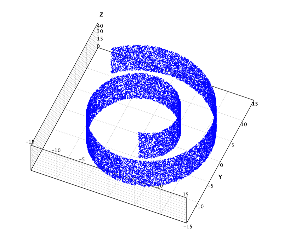

The classic Swiss roll maps 2-D points into 3-D with a smooth function so algorithms can be judged on how well they unfold the surface. The file has 20,000 samples; computing all-pairs shortest paths is expensive, so the example below uses the first 2,000 points.

import java.awt.Color;
import java.util.Arrays;
import java.util.List;
import java.util.stream.IntStream;
import org.apache.commons.csv.CSVFormat;
import smile.io.Read;
import smile.manifold.IsoMap;
import smile.graph.NearestNeighborGraph;
import smile.plot.swing.ScatterPlot;
import smile.plot.swing.Wireframe;

var swissroll = Read.csv("data/manifold/swissroll.txt",
    CSVFormat.DEFAULT.withDelimiter('\t')).toArray();
ScatterPlot.of(swissroll, '.', Color.BLUE).figure().show();

var data = Arrays.copyOf(swissroll, 2000);
var nng = NearestNeighborGraph.of(data, 7).largest(false);
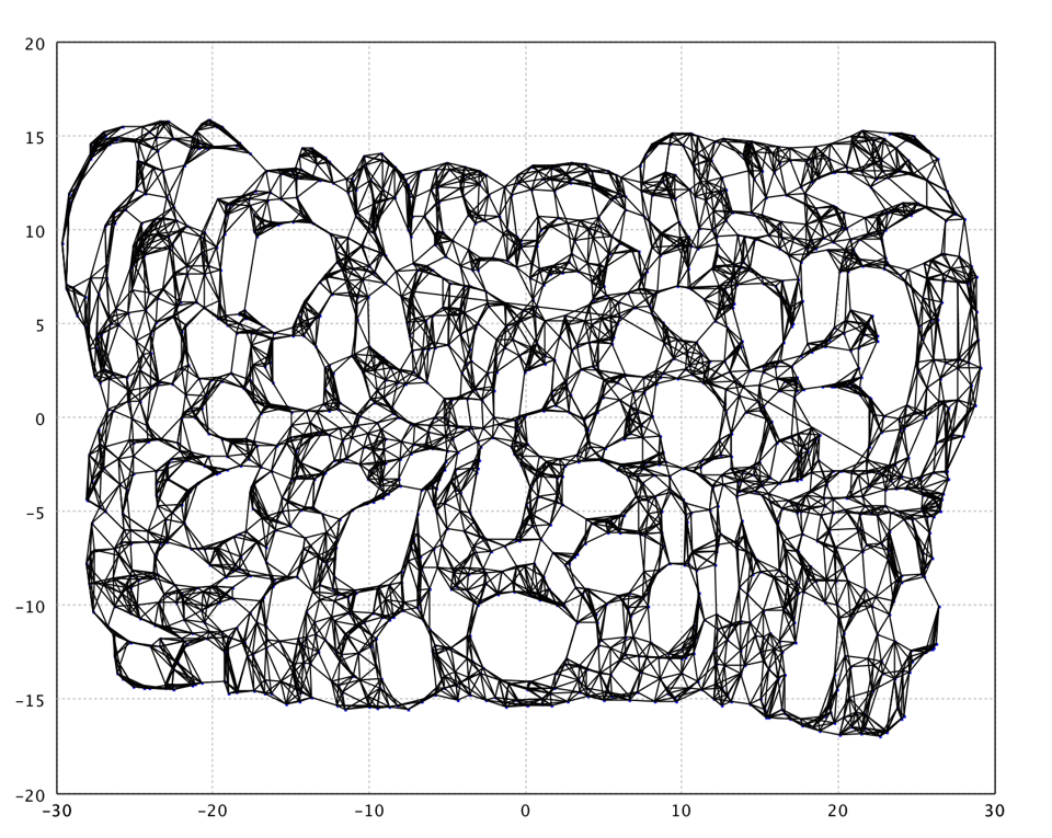
var map = IsoMap.fit(nng, new IsoMap.Options(7, 2, false));

var graph = nng.graph(false);
var edges = IntStream.range(0, data.length)
    .mapToObj(graph::getEdges)
    .flatMap(List::stream)
    .map(edge -> new int[]{edge.u(), edge.v()})
    .toArray(int[][]::new);
Wireframe.of(map, edges).figure().show();


// Wireframe / ScatterPlot windows
(opens Swiss roll and IsoMap embedding)

import smile.manifold._
import smile.plot.swing.ScatterPlot
import smile.read
import java.awt.Color.BLUE

val swissroll = read.csv("data/manifold/swissroll.txt",
  header = false, delimiter = "\t").toArray()
ScatterPlot.of(swissroll, '.', BLUE).figure.show

val data = swissroll.slice(0, 2000)
val map = isomap(data, 7, CIsomap = false)
ScatterPlot.of(map, '.', BLUE).figure.show


// Wireframe / ScatterPlot windows
(opens Swiss roll and IsoMap embedding)

import java.awt.Color
import smile.io.Read
import smile.manifold.*
import smile.plot.swing.ScatterPlot
import org.apache.commons.csv.CSVFormat

val swissroll = Read.csv("data/manifold/swissroll.txt",
    CSVFormat.DEFAULT.withDelimiter('\t')).toArray()
ScatterPlot.of(swissroll, '.', Color.BLUE).figure().show()

val data = swissroll.copyOf(2000)
val map = isomap(data, 7, CIsomap = false)
ScatterPlot.of(map, '.', Color.BLUE).figure().show()


// Wireframe / ScatterPlot windows
(opens Swiss roll and IsoMap embedding)

Here k = 7. The Java sample also draws nearest-neighbor edges in the 2-D embedding. IsoMap can leave Swiss-cheese holes; a vector-quantization pre-step often helps.

Locally Linear Embedding (LLE)

Locally Linear Embedding (LLE) finds neighbors of each point, computes weights that reconstruct the point as a linear combination of those neighbors, then solves an eigenvector problem so the same weights hold in the low-dimensional embedding. Sparse-matrix implementations make optimization fast, and results are often better than IsoMap on many problems.

When k exceeds the ambient dimension, the local Gram matrix is rank-deficient and LLE adds a small trace-proportional regularizer (factor 1E-3). LLE handles non-uniform sample density poorly — prefer Laplacian Eigenmaps or UMAP when densities vary strongly.

Hyperparameters are fields of the nested LLE.Options record. Pass an Options instance to fit, or a java.util.Properties map using the keys below (Options.toProperties() / Options.of(props) round-trip). Convenience constructor new LLE.Options(k) uses d = 2. You may also pass a pre-built NearestNeighborGraph with LLE.fit(data, nng, d).

k smile.lle.k: Number of nearest neighbors (≥ 2). Default 7.
d smile.lle.d: Embedding dimension (≥ 2). Default 2.

import smile.manifold.LLE;
import smile.graph.NearestNeighborGraph;
import smile.io.Read;
import org.apache.commons.csv.CSVFormat;
import java.util.Arrays;

var swissroll = Read.csv("data/manifold/swissroll.txt",
    CSVFormat.DEFAULT.withDelimiter('\t')).toArray();
var data = Arrays.copyOf(swissroll, 2000);

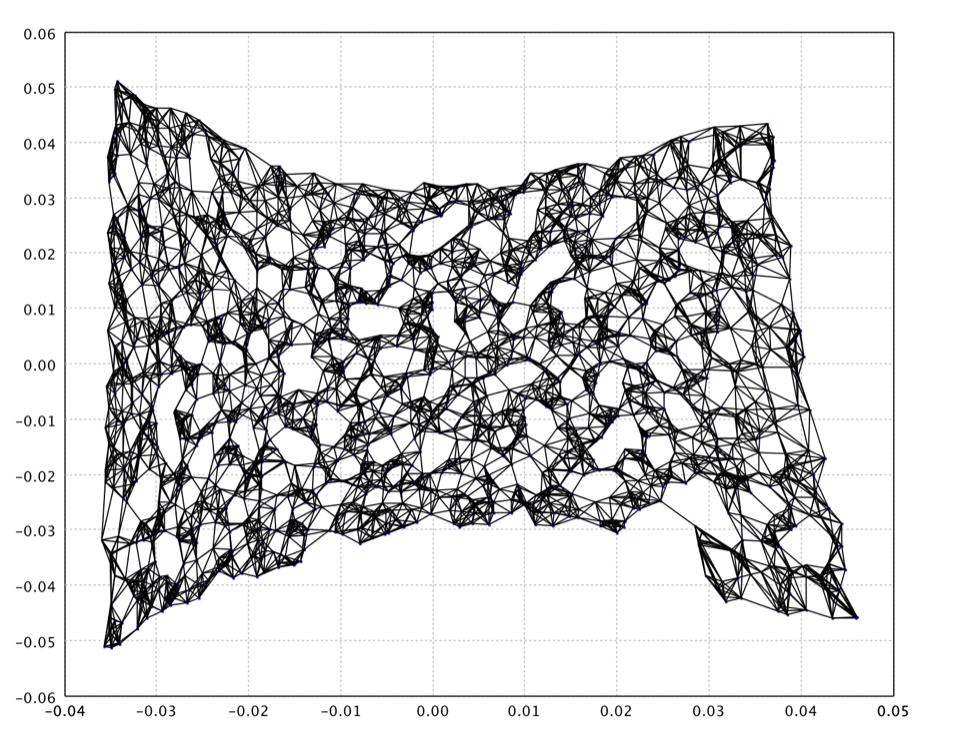
double[][] coords = LLE.fit(data, new LLE.Options(8));
NearestNeighborGraph nng = NearestNeighborGraph.of(data, 8);
double[][] fromNng = LLE.fit(data, nng, 2);


// LLE embedding of Swiss roll (k = 8)

import smile.manifold._
import smile.read

val swissroll = read.csv("data/manifold/swissroll.txt",
  header = false, delimiter = "\t").toArray()
val data = swissroll.slice(0, 2000)
val map = lle(data, 8)


// LLE embedding of Swiss roll (k = 8)

import smile.io.Read
import smile.manifold.*
import org.apache.commons.csv.CSVFormat

val swissroll = Read.csv("data/manifold/swissroll.txt",
    CSVFormat.DEFAULT.withDelimiter('\t')).toArray()
val data = swissroll.copyOf(2000)
val map = lle(data, 8)


// LLE embedding of Swiss roll (k = 8)

Laplacian Eigenmap

Laplacian Eigenmaps build a low-dimensional map that preserves local neighborhood structure via the graph Laplacian. Connected neighbors are penalized for drifting apart in the embedding. The discrete map approximates a continuous embedding that arises from the manifold’s geometry.

Two weighting schemes: discrete weights (t ≤ 0, all edges weight 1) and heat-kernel weights (t > 0): exp(−‖x_i−x_j‖² / t). Larger t yields more uniform weights; smaller t emphasizes only very close neighbors.

The method is relatively insensitive to outliers and noise and avoids short-circuiting because only local distances enter the graph. It is closely related to spectral clustering and diffusion maps.

Hyperparameters are fields of the nested LaplacianEigenmap.Options record. Pass an Options instance to fit, or a java.util.Properties map using the keys below (Options.toProperties() / Options.of(props) round-trip). Convenience constructor new LaplacianEigenmap.Options(k) uses d = 2 and t = -1.

k smile.laplacian_eigenmap.k: Number of nearest neighbors (≥ 2). Default 7.
d smile.laplacian_eigenmap.d: Embedding dimension (≥ 2). Default 2.
t smile.laplacian_eigenmap.t: Heat-kernel width. Non-positive → discrete weights. Default -1.

import smile.manifold.LaplacianEigenmap;
import smile.graph.NearestNeighborGraph;
import smile.io.Read;
import org.apache.commons.csv.CSVFormat;
import java.util.Arrays;

var swissroll = Read.csv("data/manifold/swissroll.txt",
    CSVFormat.DEFAULT.withDelimiter('\t')).toArray();
var data = Arrays.copyOf(swissroll, 2000);

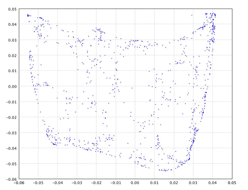
double[][] discrete = LaplacianEigenmap.fit(data,
    new LaplacianEigenmap.Options(7));
double[][] gauss = LaplacianEigenmap.fit(data,
    new LaplacianEigenmap.Options(7, 2, 25.0));

NearestNeighborGraph nng = NearestNeighborGraph.of(data, 7);
double[][] fromNng = LaplacianEigenmap.fit(nng,
    new LaplacianEigenmap.Options(7, 2, 25.0));


// Laplacian Eigenmap with heat kernel t = 25

import smile.manifold._
import smile.read

val swissroll = read.csv("data/manifold/swissroll.txt",
  header = false, delimiter = "\t").toArray()
val data = swissroll.slice(0, 2000)
val map = laplacian(data, 7, d = 2, t = 25.0)


// Laplacian Eigenmap with heat kernel t = 25

import smile.io.Read
import smile.manifold.*
import org.apache.commons.csv.CSVFormat

val swissroll = Read.csv("data/manifold/swissroll.txt",
    CSVFormat.DEFAULT.withDelimiter('\t')).toArray()
val data = swissroll.copyOf(2000)
val map = laplacian(data, 7, d = 2, t = 25.0)


// Laplacian Eigenmap with heat kernel t = 25

Kernel PCA (KPCA)

Kernel PCA applies a Mercer kernel to map data into a (possibly infinite-dimensional) feature space, then runs PCA there. Nonlinear structure that linear PCA misses can appear in the kernel principal components.

Unlike most manifold methods, KPCA implements Function<T, double[]>: call apply(newPoint) to project out-of-sample points with the same kernel. Components whose eigenvalues fall below threshold are discarded even if more than d were requested.

Hyperparameters are fields of the nested KPCA.Options record. Pass an Options instance to fit, or a java.util.Properties map using the keys below (Options.toProperties() / Options.of(props) round-trip). Convenience constructor new KPCA.Options(d) uses threshold = 1E-4.

d smile.kpca.d: Number of principal components to keep (≥ 2). Default 2.
threshold smile.kpca.threshold: Eigenvalue floor; smaller components are dropped. Default 1E-4.

import smile.manifold.KPCA;
import smile.math.kernel.GaussianKernel;
import smile.math.kernel.PolynomialKernel;
import smile.io.Read;
import org.apache.commons.csv.CSVFormat;
import java.util.Arrays;

var swissroll = Read.csv("data/manifold/swissroll.txt",
    CSVFormat.DEFAULT.withDelimiter('\t')).toArray();
var data = Arrays.copyOf(swissroll, 1000);

var kernel = new GaussianKernel(1.0);
KPCA<double[]> kpca = KPCA.fit(data, kernel, new KPCA.Options(2));
double[][] coords = kpca.coordinates();
double[] embedding = kpca.apply(data[0]);

KPCA<double[]> poly = KPCA.fit(data, new PolynomialKernel(3),
    new KPCA.Options(3));

import smile.manifold.KPCA
import smile.math.kernel.{GaussianKernel, PolynomialKernel}
import smile.read

val swissroll = read.csv("data/manifold/swissroll.txt",
  header = false, delimiter = "\t").toArray()
val data = swissroll.slice(0, 1000)

val kpca = KPCA.fit(data, new GaussianKernel(1.0), new KPCA.Options(2))
val coords = kpca.coordinates
val embedding = kpca.apply(data(0))

val poly = KPCA.fit(data, new PolynomialKernel(3), new KPCA.Options(3))

import smile.io.Read
import smile.manifold.KPCA
import smile.math.kernel.GaussianKernel
import smile.math.kernel.PolynomialKernel
import org.apache.commons.csv.CSVFormat

val swissroll = Read.csv("data/manifold/swissroll.txt",
    CSVFormat.DEFAULT.withDelimiter('\t')).toArray()
val data = swissroll.copyOf(1000)

val kpca = KPCA.fit(data, GaussianKernel(1.0), KPCA.Options(2))
val coords = kpca.coordinates()
val embedding = kpca.apply(data[0])

val poly = KPCA.fit(data, PolynomialKernel(3), KPCA.Options(3))

t-SNE

t-distributed stochastic neighbor embedding (t-SNE) is especially effective for visualizing high-dimensional data in two or three dimensions. Similar objects become nearby points; dissimilar ones become distant. High-dimensional affinities are modeled with Gaussians; the embedding uses a heavy-tailed Student-t to avoid the crowding problem. Optimization minimizes KL divergence with momentum and per-dimension adaptive gains.

If the input matrix is square, it is treated as a precomputed squared dissimilarity matrix; otherwise pairwise squared distances are computed from feature vectors. The result exposes cost() (final KL) and coordinates().

t-SNE is non-deterministic and non-parametric (no out-of-sample map). Call MathEx.setSeed before fit for reproducible layouts. Interpret plots qualitatively — 2-D distances and cluster sizes do not match the original space.

Hyperparameters are fields of the nested TSNE.Options record. Pass an Options instance to fit, or a java.util.Properties map using the keys below (Options.toProperties() / Options.of(props) round-trip). Convenience constructor new TSNE.Options(d, perplexity, eta, earlyExaggeration, maxIter) fills the remaining fields with defaults.

d smile.t_sne.d: Embedding dimension (≥ 2). Default 2.
perplexity smile.t_sne.perplexity: Effective neighborhood size (≥ 2, must be < n). Typical range 5–50. Default 20.
eta smile.t_sne.eta: Learning rate (> 0). Typical range 10–1000. Default 200.
earlyExaggeration smile.t_sne.early_exaggeration: Early-phase cluster separation (> 0). Default 12.
maxIter smile.t_sne.iterations: Maximum iterations (≥ 250). Default 1000.
maxIterWithoutProgress smile.t_sne.max_iterations_without_progress: Early-stop patience. Default 50.
tol smile.t_sne.tolerance: Gradient-norm convergence threshold. Default 1E-7.
momentum smile.t_sne.momentum: Initial momentum. Default 0.5.
finalMomentum smile.t_sne.final_momentum: Momentum after switch. Default 0.8.
momentumSwitchIter smile.t_sne.momentum_switch: Iteration to switch momentum. Default min(250, maxIter−1).
minGain smile.t_sne.min_gain: Floor for adaptive gains. Default 0.01.
controller: Optional IterativeAlgorithmController<AlgoStatus>; pass null to disable.

The MNIST example below first projects to 50 PCA dimensions, then runs t-SNE — a common speed/quality trade-off for image data.

import smile.manifold.TSNE;
import smile.feature.extraction.PCA;
import smile.io.Read;
import smile.math.MathEx;
import smile.plot.swing.ScatterPlot;
import org.apache.commons.csv.CSVFormat;

MathEx.setSeed(19650218);
var format = CSVFormat.DEFAULT.withDelimiter(' ');
var mnist = Read.csv("data/mnist/mnist2500_X.txt", format).toArray();
var label = Read.csv("data/mnist/mnist2500_labels.txt", format)
    .column(0).toIntArray();

var pca = PCA.fit(mnist).getProjection(50);
var X = pca.apply(mnist);
var tsne = TSNE.fit(X, new TSNE.Options(2, 20, 200, 12, 1000));

var figure = ScatterPlot.of(tsne.coordinates(), label, '@').figure();
figure.setTitle("t-SNE of MNIST");
figure.show();


// ScatterPlot.of(tsne.coordinates(), label, '@').figure().show()
(opens t-SNE of MNIST)

import smile.manifold._
import smile.feature.extraction.PCA
import smile.math.MathEx
import smile.plot.swing.ScatterPlot
import smile.read

MathEx.setSeed(19650218)
val mnist = read.csv("data/mnist/mnist2500_X.txt",
  header = false, delimiter = " ").toArray()
val label = read.csv("data/mnist/mnist2500_labels.txt",
  header = false, delimiter = " ").column(0).toIntArray()

val pc = PCA.fit(mnist).getProjection(50)
val x50 = pc.apply(mnist)
val sne = tsne(x50, d = 2, perplexity = 20, eta = 200, maxIter = 1000)

val figure = ScatterPlot.of(sne.coordinates, label, '@').figure
figure.setTitle("t-SNE of MNIST")
figure.show


// ScatterPlot.of(tsne.coordinates(), label, '@').figure().show()
(opens t-SNE of MNIST)

import smile.io.Read
import smile.manifold.*
import smile.feature.extraction.PCA
import smile.math.MathEx
import smile.plot.swing.ScatterPlot
import org.apache.commons.csv.CSVFormat

MathEx.setSeed(19650218)
val format = CSVFormat.DEFAULT.withDelimiter(' ')
val mnist = Read.csv("data/mnist/mnist2500_X.txt", format).toArray()
val label = Read.csv("data/mnist/mnist2500_labels.txt", format)
    .column(0).toIntArray()

val pc = PCA.fit(mnist).getProjection(50)
val x50 = pc.apply(mnist)
val sne = tsne(x50, d = 2, perplexity = 20.0, eta = 200.0, maxIter = 1000)

val figure = ScatterPlot.of(sne.coordinates(), label, '@').figure()
figure.setTitle("t-SNE of MNIST")
figure.show()


// ScatterPlot.of(tsne.coordinates(), label, '@').figure().show()
(opens t-SNE of MNIST)

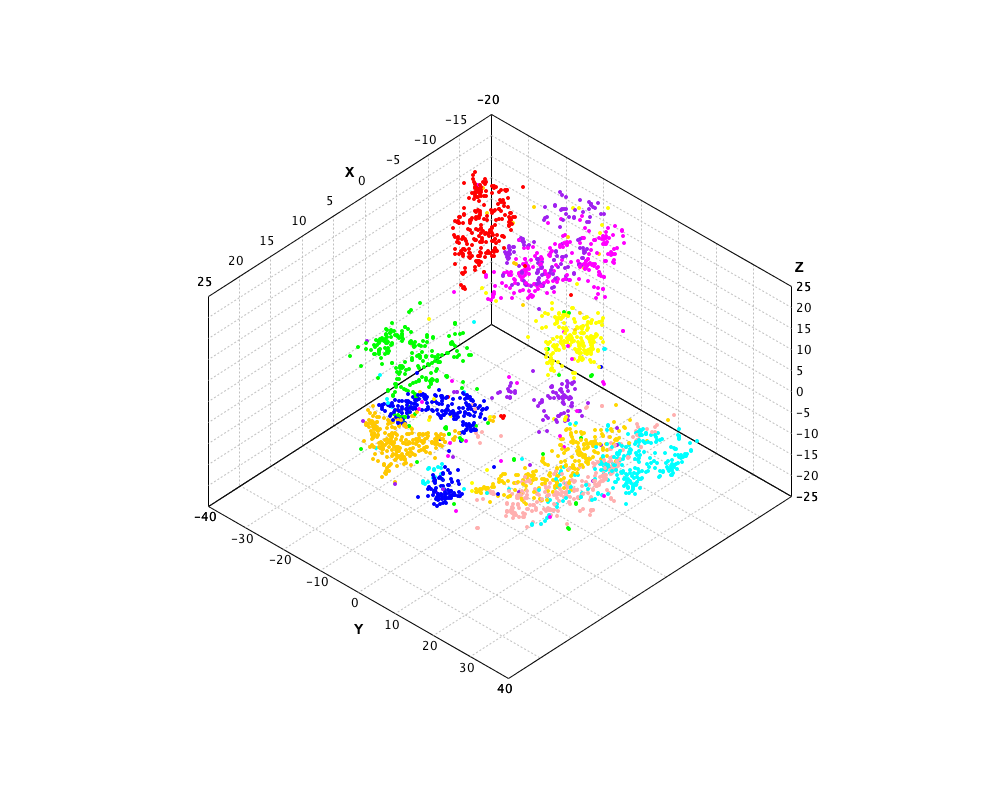
UMAP

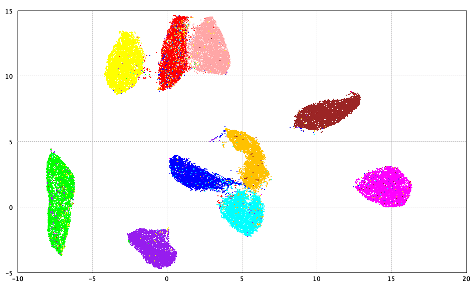
Uniform Manifold Approximation and Projection can visualize data like t-SNE and also serve as general nonlinear dimension reduction. It assumes the data are uniformly distributed on a Riemannian manifold, the metric is locally approximately constant, and the manifold is locally connected. From those assumptions it builds a fuzzy topological model and finds a low-dimensional layout with matching topology.

Euclidean distance by default, or any custom Metric<T>.
If epochs = 0, SMILE picks 500 epochs for small data (< 10,000 points) and 200 for large.
For more than 10,000 points, approximate NNG via NearestNeighborGraph.descent() avoids O(n²) exact construction.

Hyperparameters are fields of the nested UMAP.Options record. Pass an Options instance to fit, or a java.util.Properties map using the keys below (Options.toProperties() / Options.of(props) round-trip). Convenience constructor new UMAP.Options(k) uses d = 2, auto epochs, and the defaults above. UMAP is non-deterministic; fix MathEx.setSeed for reproducibility.

k smile.umap.k: Nearest neighbors (≥ 2). Larger → more global view. Default 15.
d smile.umap.d: Embedding dimension (≥ 2). Default 2.
epochs smile.umap.epochs: Optimization epochs; 0 = auto (200 or 500). Default 0.
learningRate smile.umap.learning_rate: Initial learning rate (> 0). Default 1.0.
minDist smile.umap.min_dist: Minimum distance between embedded points (> 0, ≤ spread). Smaller → tighter clusters. Default 0.1.
spread smile.umap.spread: Scale of the embedded space. Default 1.0.
negativeSamples smile.umap.negative_samples: Negative samples per positive sample (> 0). Default 5.
repulsionStrength smile.umap.repulsion_strength: Weight of repulsion forces. Default 1.0.
localConnectivity smile.umap.local_connectivity: Required local connectivity (≥ 1). Default 1.0.

import smile.manifold.UMAP;
import smile.math.MathEx;
import smile.io.Read;
import smile.plot.swing.ScatterPlot;
import org.apache.commons.csv.CSVFormat;

MathEx.setSeed(19650218);
var format = CSVFormat.DEFAULT.withDelimiter(' ');
var mnist = Read.csv("data/mnist/mnist2500_X.txt", format).toArray();
var label = Read.csv("data/mnist/mnist2500_labels.txt", format)
    .column(0).toIntArray();

var map = UMAP.fit(mnist, new UMAP.Options(15));
ScatterPlot.of(map, label, '@').figure().show();


// ScatterPlot.of(map, label, '@').figure().show()
(opens UMAP of MNIST)

import smile.manifold._
import smile.math.MathEx
import smile.plot.swing.ScatterPlot
import smile.read

MathEx.setSeed(19650218)
val mnist = read.csv("data/mnist/mnist2500_X.txt",
  header = false, delimiter = " ").toArray()
val label = read.csv("data/mnist/mnist2500_labels.txt",
  header = false, delimiter = " ").column(0).toIntArray()

val map = umap(mnist, k = 15)
ScatterPlot.of(map, label, 'o').figure.show


// ScatterPlot.of(map, label, '@').figure().show()
(opens UMAP of MNIST)

import smile.io.Read
import smile.manifold.*
import smile.math.MathEx
import smile.plot.swing.ScatterPlot
import org.apache.commons.csv.CSVFormat

MathEx.setSeed(19650218)
val format = CSVFormat.DEFAULT.withDelimiter(' ')
val mnist = Read.csv("data/mnist/mnist2500_X.txt", format).toArray()
val label = Read.csv("data/mnist/mnist2500_labels.txt", format)
    .column(0).toIntArray()

val map = umap(mnist, k = 15)
ScatterPlot.of(map, label, '@').figure().show()


// ScatterPlot.of(map, label, '@').figure().show()
(opens UMAP of MNIST)

Tips and Best Practices

Pre-process. Standardize features (or use a robust scaler) so no single coordinate dominates distances. For images, a PCA reduction to 50–100 dimensions before t-SNE or UMAP usually helps speed without much loss.
Neighborhood size k. Smaller values keep fine local structure but are noise-sensitive; larger values smooth globally but may bridge clusters. Starting ranges: LLE / Laplacian 5–15, IsoMap 7–15, UMAP 10–30.
t-SNE perplexity. Try ≈ √n as a start; always keep perplexity < n. Different values reveal structure at different scales.
UMAP minDist. Use ~0.01–0.1 for tight clusters; raise toward 0.3+ for continuous trajectories.
Disconnected graphs. IsoMap, LLE, and Laplacian use only the largest connected component. If points drop out, increase k.
Reproducibility. MathEx.setSeed(…) before t-SNE or UMAP.

← Multi-Dimensional Scaling Large Language Models →