Interpolation
Interpolation builds a function that passes through given samples so you
can evaluate it between the knots. SMILE’s
smile.interpolation
package covers 1-D and 2-D methods behind
Interpolation and Interpolation2D
(interpolate(...)).
Examples below reuse a short sample of sin(x) at integer
knots 0…6. Plot snippets open a Swing window; the static
figures show the same curves.
Piecewise Linear Interpolation
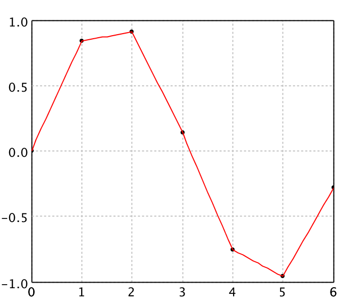
LinearInterpolation is fast and simple, but the interpolant
is only C0 (not differentiable at the knots).
BilinearInterpolation extends the idea to a regular 2-D
grid by interpolating once in each direction.
import java.awt.Color
import smile.interpolation.LinearInterpolation
import smile.plot.swing.*

double[] x = {0.0, 1.0, 2.0, 3.0, 4.0, 5.0, 6.0}
double[] y = {0.0, 0.8415, 0.9093, 0.1411, -0.7568, -0.9589, -0.2794}
double[][] points = new double[x.length][2]
for (int i = 0; i < x.length; i++) {
    points[i][0] = x[i]
    points[i][1] = y[i]
}

var linear = new LinearInterpolation(x, y)
linear.interpolate(2.5)

double[][] curve = new double[61][2]
for (int i = 0; i < curve.length; i++) {
    curve[i][0] = i * 0.1
    curve[i][1] = linear.interpolate(curve[i][0])
}
var figure = ScatterPlot.of(points, '@', Color.BLACK).figure()
figure.add(LinePlot.of(curve, Color.RED))
figure.show()
0.5252
(opens plot: knots + red piecewise-linear curve)
import java.awt.Color
import smile.interpolation.LinearInterpolation
import smile.plot.swing.LinePlot

val x = Array(0.0, 1.0, 2.0, 3.0, 4.0, 5.0, 6.0)
val y = Array(0.0, 0.8415, 0.9093, 0.1411, -0.7568, -0.9589, -0.2794)
val points = x.indices.map(i => Array(x(i), y(i))).toArray

val linear = new LinearInterpolation(x, y)
linear.interpolate(2.5)

val curve = (0 to 60).map { i =>
  val xi = i * 0.1
  Array(xi, linear.interpolate(xi))
}.toArray

val canvas = plot(points, '@', Color.BLACK)
canvas.figure().add(LinePlot.of(curve, Color.RED))
show(canvas)
0.5252
(opens plot: knots + red piecewise-linear curve)
Cubic Spline Interpolation
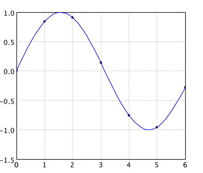
Natural cubic splines are piecewise cubics that are C2, with zero second derivative at the endpoints. They avoid Runge’s phenomenon of high-degree global polynomials while staying easy to evaluate.
import java.awt.Color
import smile.interpolation.CubicSplineInterpolation1D
import smile.plot.swing.*

double[] x = {0.0, 1.0, 2.0, 3.0, 4.0, 5.0, 6.0}
double[] y = {0.0, 0.8415, 0.9093, 0.1411, -0.7568, -0.9589, -0.2794}
double[][] points = new double[x.length][2]
for (int i = 0; i < x.length; i++) {
    points[i][0] = x[i]
    points[i][1] = y[i]
}

var cubic = new CubicSplineInterpolation1D(x, y)
cubic.interpolate(2.5)

double[][] curve = new double[61][2]
for (int i = 0; i < curve.length; i++) {
    curve[i][0] = i * 0.1
    curve[i][1] = cubic.interpolate(curve[i][0])
}
var figure = ScatterPlot.of(points, '@', Color.BLACK).figure()
figure.add(LinePlot.of(curve, Color.BLUE))
figure.show()
0.5962098076923077
(opens plot: knots + blue cubic spline)
import java.awt.Color
import smile.interpolation.CubicSplineInterpolation1D
import smile.plot.swing.LinePlot

val x = Array(0.0, 1.0, 2.0, 3.0, 4.0, 5.0, 6.0)
val y = Array(0.0, 0.8415, 0.9093, 0.1411, -0.7568, -0.9589, -0.2794)
val points = x.indices.map(i => Array(x(i), y(i))).toArray

val cubic = new CubicSplineInterpolation1D(x, y)
cubic.interpolate(2.5)

val curve = (0 to 60).map { i =>
  val xi = i * 0.1
  Array(xi, cubic.interpolate(xi))
}.toArray

val canvas = plot(points, '@', Color.BLACK)
canvas.figure().add(LinePlot.of(curve, Color.BLUE))
show(canvas)
0.5962098076923077
(opens plot: knots + blue cubic spline)
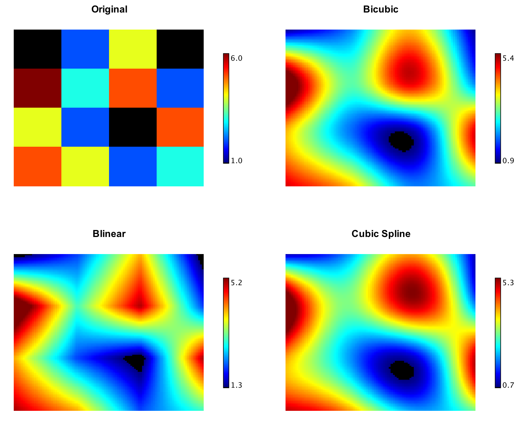
On a regular 2-D grid,
CubicSplineInterpolation2D keeps first and second
derivatives continuous;
BicubicInterpolation guarantees continuity of the
gradient and cross-derivative only (often enough for image resampling).
import smile.interpolation.*
import smile.plot.swing.*

double[] x1 = {1950.0, 1960, 1970, 1980, 1990}
double[] x2 = {10.0, 20, 30}
double[][] y = {
    {150.697, 199.592, 187.625},
    {179.323, 195.072, 250.287},
    {203.212, 179.092, 322.767},
    {226.505, 153.706, 426.730},
    {249.633, 120.281, 598.243}
}

Heatmap.of(y, Palette.jet(256)).figure().setTitle("Original").show()

var cubic = new CubicSplineInterpolation2D(x1, x2, y)
var bicubic = new BicubicInterpolation(x1, x2, y)
cubic.interpolate(1975, 15)
bicubic.interpolate(1975, 15)

double[][] data = new double[101][101]
for (int i = 0; i <= 100; i++)
    for (int j = 0; j <= 100; j++)
        data[i][j] = cubic.interpolate(1950 + i * 0.4, 10 + j * 0.2)
Heatmap.of(data, Palette.jet(256)).figure().setTitle("Cubic").show()

for (int i = 0; i <= 100; i++)
    for (int j = 0; j <= 100; j++)
        data[i][j] = bicubic.interpolate(1950 + i * 0.4, 10 + j * 0.2)
Heatmap.of(data, Palette.jet(256)).figure().setTitle("Bicubic").show()
167.9922755301339   // cubic at (1975, 15)
175.6672890625      // bicubic at (1975, 15)
(opens Original / Cubic / Bicubic heatmaps)
import smile.interpolation.*
import smile.plot.swing.Palette

val x1 = Array(1950.0, 1960, 1970, 1980, 1990)
val x2 = Array(10.0, 20, 30)
val y = Array(
  Array(150.697, 199.592, 187.625),
  Array(179.323, 195.072, 250.287),
  Array(203.212, 179.092, 322.767),
  Array(226.505, 153.706, 426.730),
  Array(249.633, 120.281, 598.243)
)

val original = heatmap(y, Palette.jet(256))
original.figure().setTitle("Original")
show(original)

val cubic = new CubicSplineInterpolation2D(x1, x2, y)
val bicubic = new BicubicInterpolation(x1, x2, y)
cubic.interpolate(1975, 15)
bicubic.interpolate(1975, 15)

val data = Array.ofDim[Double](101, 101)
for (i <- 0 to 100; j <- 0 to 100)
  data(i)(j) = cubic.interpolate(1950 + i * 0.4, 10 + j * 0.2)
val cubicPlot = heatmap(data, Palette.jet(256))
cubicPlot.figure().setTitle("Cubic")
show(cubicPlot)

for (i <- 0 to 100; j <- 0 to 100)
  data(i)(j) = bicubic.interpolate(1950 + i * 0.4, 10 + j * 0.2)
val bicubicPlot = heatmap(data, Palette.jet(256))
bicubicPlot.figure().setTitle("Bicubic")
show(bicubicPlot)
167.9922755301339   // cubic at (1975, 15)
175.6672890625      // bicubic at (1975, 15)
(opens Original / Cubic / Bicubic heatmaps)
Kriging Interpolation
Ordinary kriging (Gauss–Markov / Gaussian-process regression with a
power variogram) works for irregularly spaced samples in 1-D or 2-D
(KrigingInterpolation1D, KrigingInterpolation2D,
KrigingInterpolation).
import java.awt.Color
import smile.interpolation.KrigingInterpolation1D
import smile.plot.swing.*

double[] x = {0.0, 1.0, 2.0, 3.0, 4.0, 5.0, 6.0}
double[] y = {0.0, 0.8415, 0.9093, 0.1411, -0.7568, -0.9589, -0.2794}
double[][] points = new double[x.length][2]
for (int i = 0; i < x.length; i++) {
    points[i][0] = x[i]
    points[i][1] = y[i]
}

var kriging = new KrigingInterpolation1D(x, y)
kriging.interpolate(2.5)

double[][] curve = new double[61][2]
for (int i = 0; i < curve.length; i++) {
    curve[i][0] = i * 0.1
    curve[i][1] = kriging.interpolate(curve[i][0])
}
var figure = ScatterPlot.of(points, '@', Color.BLACK).figure()
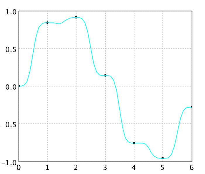
figure.add(LinePlot.of(curve, Color.CYAN))
figure.show()
0.5696185426834837
(opens plot: knots + cyan kriging curve)
import java.awt.Color
import smile.interpolation.KrigingInterpolation1D
import smile.plot.swing.LinePlot

val x = Array(0.0, 1.0, 2.0, 3.0, 4.0, 5.0, 6.0)
val y = Array(0.0, 0.8415, 0.9093, 0.1411, -0.7568, -0.9589, -0.2794)
val points = x.indices.map(i => Array(x(i), y(i))).toArray

val kriging = new KrigingInterpolation1D(x, y)
kriging.interpolate(2.5)

val curve = (0 to 60).map { i =>
  val xi = i * 0.1
  Array(xi, kriging.interpolate(xi))
}.toArray

val canvas = plot(points, '@', Color.BLACK)
canvas.figure().add(LinePlot.of(curve, Color.CYAN))
show(canvas)
0.5696185426834837
(opens plot: knots + cyan kriging curve)
RBF Interpolation
Radial basis function interpolants take the form
y(x) = Σ wi φ(‖x − ci‖).
Centers need not lie on a grid; weights come from a linear least-squares
solve. Common kernels in
smile.math.rbf
include Gaussians, multiquadrics, inverse multiquadrics, and thin-plate
splines (shape parameter r0 controls flatness /
conditioning). A normalized RBF (NRBF) variant forces the basis
functions to sum to one.
import java.awt.Color
import smile.interpolation.RBFInterpolation1D
import smile.math.rbf.GaussianRadialBasis
import smile.plot.swing.*

double[] x = {0.0, 1.0, 2.0, 3.0, 4.0, 5.0, 6.0}
double[] y = {0.0, 0.8415, 0.9093, 0.1411, -0.7568, -0.9589, -0.2794}
double[][] points = new double[x.length][2]
for (int i = 0; i < x.length; i++) {
    points[i][0] = x[i]
    points[i][1] = y[i]
}

var rbf = new RBFInterpolation1D(x, y, new GaussianRadialBasis())
rbf.interpolate(2.5)

double[][] curve = new double[61][2]
for (int i = 0; i < curve.length; i++) {
    curve[i][0] = i * 0.1
    curve[i][1] = rbf.interpolate(curve[i][0])
}
var figure = ScatterPlot.of(points, '@', Color.BLACK).figure()
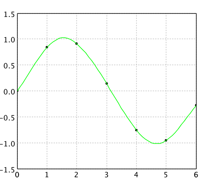
figure.add(LinePlot.of(curve, Color.GREEN))
figure.show()
0.5806031141431599
(opens plot: knots + green Gaussian RBF curve)
import java.awt.Color
import smile.interpolation.RBFInterpolation1D
import smile.math.rbf.GaussianRadialBasis
import smile.plot.swing.LinePlot

val x = Array(0.0, 1.0, 2.0, 3.0, 4.0, 5.0, 6.0)
val y = Array(0.0, 0.8415, 0.9093, 0.1411, -0.7568, -0.9589, -0.2794)
val points = x.indices.map(i => Array(x(i), y(i))).toArray

val rbf = new RBFInterpolation1D(x, y, new GaussianRadialBasis())
rbf.interpolate(2.5)

val curve = (0 to 60).map { i =>
  val xi = i * 0.1
  Array(xi, rbf.interpolate(xi))
}.toArray

val canvas = plot(points, '@', Color.BLACK)
canvas.figure().add(LinePlot.of(curve, Color.GREEN))
show(canvas)
0.5806031141431599
(opens plot: knots + green Gaussian RBF curve)
Shepard Interpolation
Shepard interpolation is a normalized RBF special case with
φ(r) = r−p (typically 1 < p ≤ 3).
Weights equal the observed values, so no linear system is solved and
large N is cheap—often “quick and dirty” rather than
highest accuracy. See also
ShepardInterpolation2D for scattered 2-D data.
import java.awt.Color
import smile.interpolation.ShepardInterpolation1D
import smile.plot.swing.*

double[] x = {0.0, 1.0, 2.0, 3.0, 4.0, 5.0, 6.0}
double[] y = {0.0, 0.8415, 0.9093, 0.1411, -0.7568, -0.9589, -0.2794}
double[][] points = new double[x.length][2]
for (int i = 0; i < x.length; i++) {
    points[i][0] = x[i]
    points[i][1] = y[i]
}

var shepard = new ShepardInterpolation1D(x, y, 3)
shepard.interpolate(2.5)

double[][] curve = new double[61][2]
for (int i = 0; i < curve.length; i++) {
    curve[i][0] = i * 0.1
    curve[i][1] = shepard.interpolate(curve[i][0])
}
var figure = ScatterPlot.of(points, '@', Color.BLACK).figure()
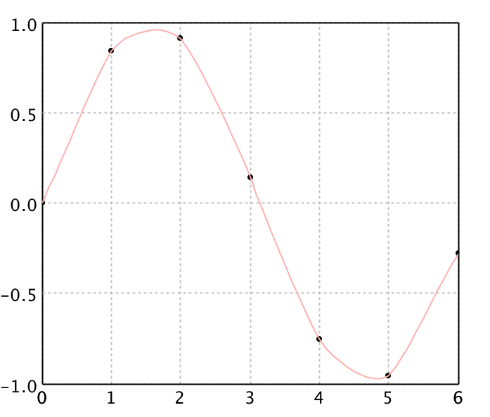
figure.add(LinePlot.of(curve, Color.PINK))
figure.show()
0.4993103151310187
(opens plot: knots + pink Shepard curve)
import java.awt.Color
import smile.interpolation.ShepardInterpolation1D
import smile.plot.swing.LinePlot

val x = Array(0.0, 1.0, 2.0, 3.0, 4.0, 5.0, 6.0)
val y = Array(0.0, 0.8415, 0.9093, 0.1411, -0.7568, -0.9589, -0.2794)
val points = x.indices.map(i => Array(x(i), y(i))).toArray

val shepard = new ShepardInterpolation1D(x, y, 3)
shepard.interpolate(2.5)

val curve = (0 to 60).map { i =>
  val xi = i * 0.1
  Array(xi, shepard.interpolate(xi))
}.toArray

val canvas = plot(points, '@', Color.BLACK)
canvas.figure().add(LinePlot.of(curve, Color.PINK))
show(canvas)
0.4993103151310187
(opens plot: knots + pink Shepard curve)
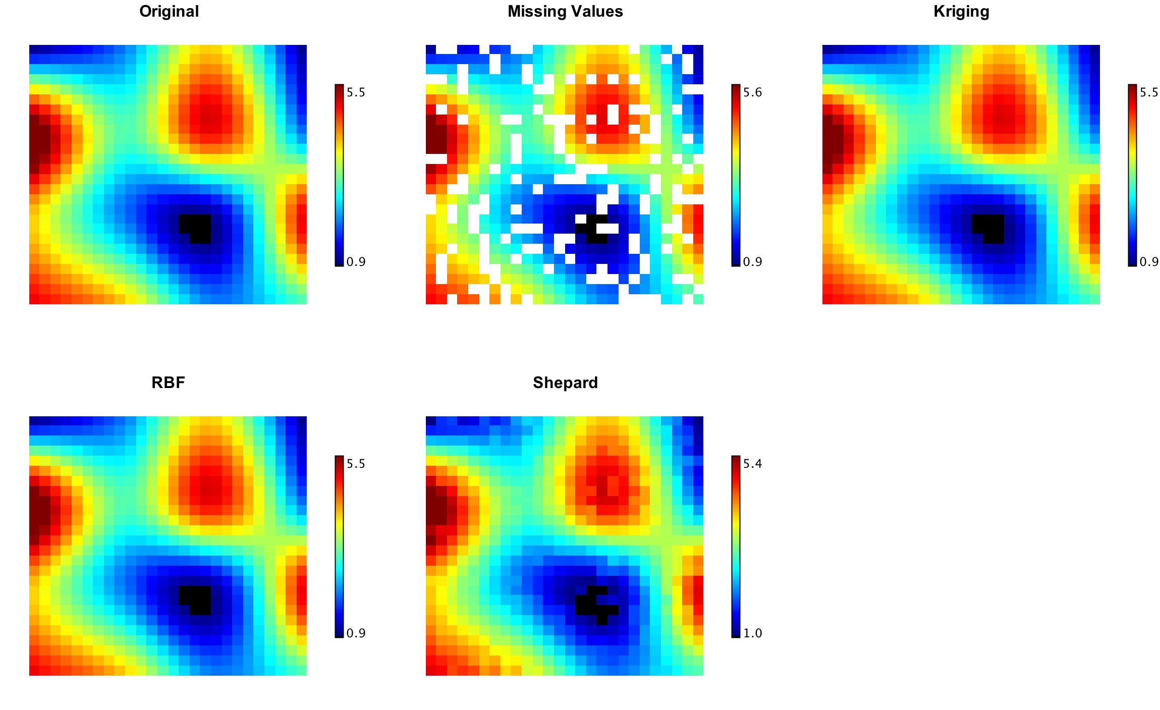
Scattered 2-D methods (kriging / RBF / Shepard) on irregular samples.
Laplace Interpolation
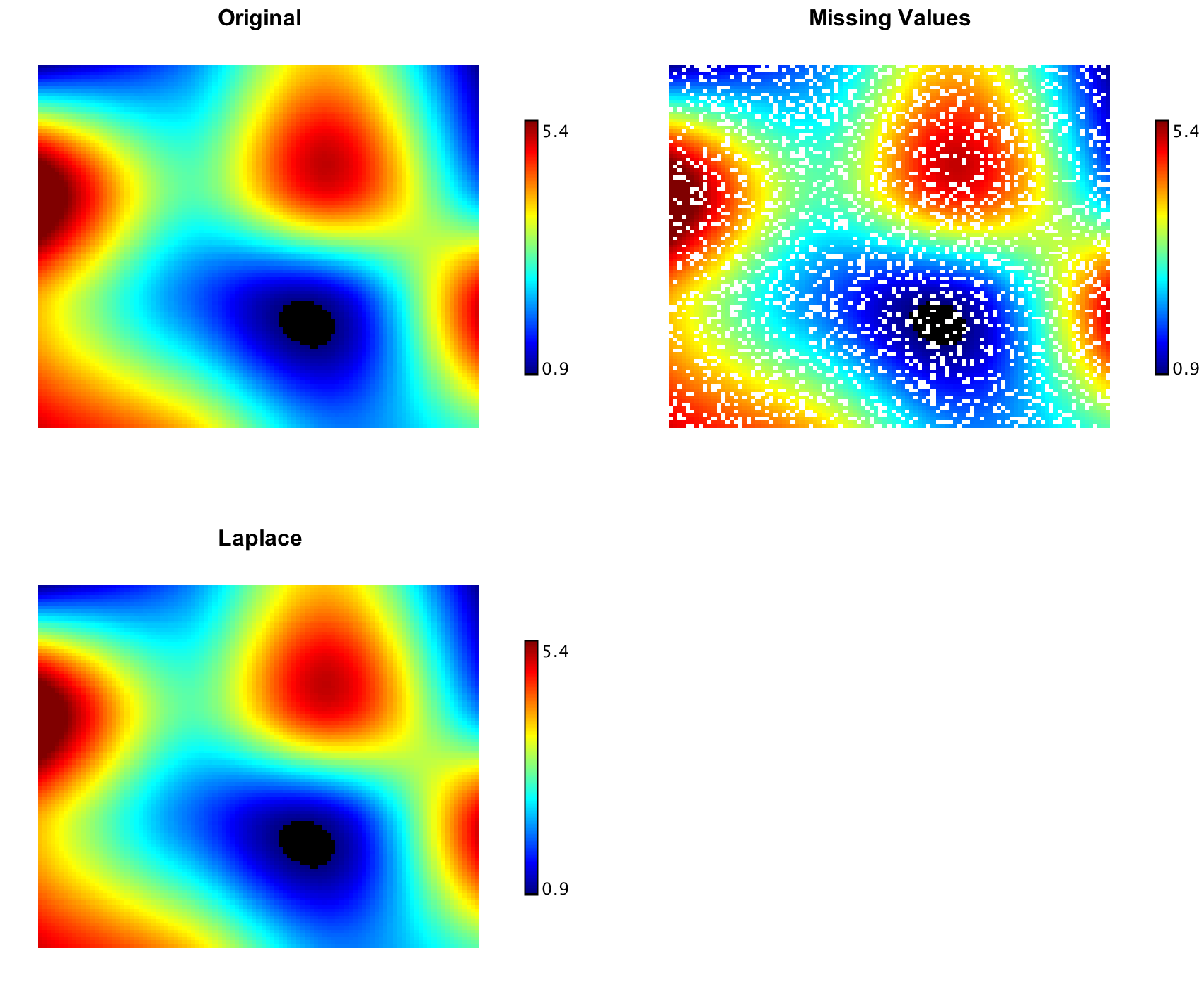
LaplaceInterpolation fills NaN entries on a
regular 2-D grid by solving a sparse Laplace equation (biconjugate
gradient)—a smooth way to restore missing measurements.
import smile.interpolation.LaplaceInterpolation
import smile.math.MathEx
import smile.plot.swing.*

MathEx.setSeed(19650218)
double[][] grid = new double[41][41]
for (int i = 0; i < 41; i++)
    for (int j = 0; j < 41; j++)
        grid[i][j] = Math.sin(i / 6.0) * Math.cos(j / 6.0)

double[][] missing = new double[41][41]
for (int i = 0; i < 41; i++)
    for (int j = 0; j < 41; j++)
        missing[i][j] = MathEx.random() < 0.25 ? Double.NaN : grid[i][j]

Heatmap.of(missing, Palette.jet(256)).figure().setTitle("Missing Values").show()
double err = LaplaceInterpolation.interpolate(missing)
Heatmap.of(missing, Palette.jet(256)).figure().setTitle("Laplace").show()
err
(opens Missing Values / Laplace heatmaps)
err ≈ residual of the sparse solve (small)
import smile.interpolation.LaplaceInterpolation
import smile.math.MathEx
import smile.plot.swing.Palette

MathEx.setSeed(19650218)
val grid = Array.tabulate(41, 41) { (i, j) =>
  Math.sin(i / 6.0) * Math.cos(j / 6.0)
}
val missing = Array.tabulate(41, 41) { (i, j) =>
  if (MathEx.random() < 0.25) Double.NaN else grid(i)(j)
}

val missPlot = heatmap(missing, Palette.jet(256))
missPlot.figure().setTitle("Missing Values")
show(missPlot)

val err = LaplaceInterpolation.interpolate(missing)
val filled = heatmap(missing, Palette.jet(256))
filled.figure().setTitle("Laplace")
show(filled)
err
(opens Missing Values / Laplace heatmaps)
err ≈ residual of the sparse solve (small)